Introduction to PyTorch

What is PyTorch?

PyTorch is an open-source deep-learning library based on Torch, a framework for scientific computing.

• With most of it written in C++ and CUDA, PyTorch offers high-performance and efficient scientific computing through its core data structure called tensors.
• It is flexible in its use, highly customizable, and thus allows for the implementation of novel neural architectures with ease.
• It has tensor as its core data structure; tensors are highly similar to (multidimensional) NumPy arrays and have the support/ability to run on GPUs for faster computation.

Features of PyTorch

1. Use in Python - PyTorch can be run with C++ as well; however, its easy use and integration with the Python ecosystem, along with the pythonic nature of the library, makes it a go-to choice for Deep learning research professionals as well as academicians.

2. Domain-specific features - PyTorch consists of packages that are useful for various domains where Deep Learning could be applied. For example - torchtext offers various text processing functionalities and popular data sets for natural language processing, torchaudio offers utilities for audio and signal processing so on and so forth.

3. Cloud support - Pytorch is supported on all major cloud platforms allowing for easy and scalable development of Machine Learning systems, along with the support to deploy them in production.

4. Native Deployment Tools - With its growing user base, PyTorch is swiftly bridging the gap where it initially lacked in, that is, the availability of and easy access to robust deployment tools. PyTorch now has its native deployment tools called TorchServe and PyTorch Lite.

Advantages of Pytorch

1. Tensors and the wide functionality - Optimised and efficiently fast mathematical operations could be done using PyTorch tensors on both GPU and CPU. The shift from CPU to GPU is readily done and is just one or two function calls. Moreover, PyTorch can automatically keep track of all the operations that are performed on tensors and thus offers automatic calculation of gradients which are the backbone of training deep neural networks.

2. Flexibility and customizability - PyTorch offers a plethora of loss functions for defining training criteria, along with various layers and activation functions to specify and define custom neural network architectures. The easy access to low-level features is a boon for deep learning research when it comes to implementing novel architectures. Thus it offers the best of both worlds by offering access to low-level features along with making them super easy to implement and build.

3. Speed of computation - Pytorch has support for and compatibility with NVIDIA's CUDA-based GPUs that accelerate the training of neural networks by many orders of magnitude. Apart from this, distributed training offered by the library could parallelize operations across multiple GPUs and thus make the training process even faster.

Basic Tensor Operations with PyTorch

What are Tensors?

Tensors are the core data structures of PyTorch; very similar to NumPy ndarrays, tensors are also multidimensional array-like structures and come with additional functionalities like their ability to run on GPUs and be referenced by computation graphs that internally help PyTorch calculate gradients for the training of deep learning networks.

Tensors, unlike NumPy arrays, have special attributes associated with them that are mostly concerned with gradient calculations and computational graphs. We will see and talk about almost all of these attributes later in the article when we walk through autograd.

Creation of Tensors and Major Operations

Here are some common ways to create tensors in Pytorch -

Output:

Apart from the ones above, there are other commonly used ways to create tensors like torch.randn(), torch.randperm(), torch.ones(), torch.zeros(), and so on.

Or, we could also use numpy arrays to create pytorch tensors while leveraging the interoperability between the two, like so-

Output:

Notice how the tensors and the numpy arrays share the same storage location in the memory and changing one hence changes the other, which is why a change in array b changed tensor t.

Tensors also have the data type attribute as dtype that lets us specify the desired precision for our operations, like so -

Output:

The operations on Pytorch tensors are very similar to those on numpy arrays like so -

Checking size of tensors -

Output:

Adding tensors -

Output:

Or, using in-place operations, like so -

Output:

Reshaping tensors

Deep neural networks require the data to be inputted in a specific shape/ dimensionality. For example, one network might want the input image to be 3-dimensional - one dimension for the color channels and the other two representing the height and width of the image.

On the other hand, another network might expect two dimensions for an image tensor - one representing the colour channel and the other one representing pixels as one long vector so that a 25 * 25 image becomes an array containing 125 values.

To this end, PyTorch provides easy ways to reshape our input tensor data, some of which are discussed -

1. PyTorch reshape - torch.reshape(input, shape) Reshapes the input to the specified shape and returns the reshaped tensor. It is important to note that reshape can return tensors that are either copies of the original tensor reshaped accordingly or just a view on the original tensor, in which case any changes made in the output tensor shall reflect in the input tensor, like so-

Output:

However, it's better to use reshape when it is not possible to return views on the original tensor.

2. PyTorch view - torch.tensor.view(*shape) Returns a view of the original tensor in the desired shape. No data is copied here, and using a view on tensors is only possible when the specified shape is compatible with the original tensor's shape and stride. When using view is possible, it is advised to use view only and not reshape.

Output:

3. PyTorch flatten - torch.flatten(input, start_dim=0, end_dim=- 1) Returns a tensor by flattening the input tensor starting with start_dim and ending with end_dim. If default values are used, the returned tensor is one-dimensional. Like reshaping, it also provides a view if possible else the data is copied.

Output:

4. PyTorch permute - torch.permute(input, dims) permute returns a view of the original tensor input with the returned tensor having its dimensions permuted, like so-

Output:

Some more operations

PyTorch unsqueeze - torch.unsqueeze(input, dim):

unsqueeze returns a new tensor sharing the same data with the input tensor but a dimension of size one inserted at the dim position. So, let's say we have a tensor of size torch.Size([2, 3]), and we want to get another tensor having the same data as this one but with size torch.Size([1, 2, 3]) - here, we could use unsqueeze to insert a dimension of size one at dim=0.Let's see this happening via some code:

Output:

PyTorch detach - torch.detach():

detach detaches a tensor from its computation graph, thus returning a new tensor that shares the same storage as the input tensor but has its requires_grad attribute set to False.

detach has many use cases - it gives the ability to be able to control model gradients during the training procedure. In one single iteration, a model might need gradients for one purpose and might not need them for some other purpose. In the latter case, we could detach the tensors to stop the expensive gradient calculations.

Let's see detach in action -

Output:

Another potential use of torch.detach is as follows - Let's say a particular tensor representing the loss of a complex architecture is required outside of the training loop as well. But only the value of this loss is required, say for printing or storing it somewhere later in the code.

As the loss tensor would already have a computation graph associated with it inside the training loop due to it being subjected to a variety of mathematical operations, this graph shall continue to hang around in the memory as long as we keep this tensor in the memory.

Even after backward calls are made in the training loop, this graph keeps lingering in the memory.

For this graph to get garbage collected as it isn't needed anymore, we could just detach the loss tensor from it and hence save the memory.

Automatic Differentiation

Some terms: Before defining the autograd engine, we'll first briefly look at three basic terms used in the deep learning space -

• Loss function - The difference between the expected model output and the actual output produced by the model is called the loss function. Loss function is the one that we aim to minimize during the training of neural networks so as to get the model outputs as close to the expected (desired) outputs as possible.

• Gradient Descent - To minimize the loss function, the model parameters (weights and biases) are updated iteratively by moving in the negative direction of the steepest gradient. Mathematically, this amounts to taking the negative of the gradients of the loss function with respect to the different parameters of the model that need to be optimized. This optimization algorithm aimed at reaching local minima in the loss landscape is called the gradient descent algorithm.

• Backpropagation - Backpropagation of gradients is at the heart of training most deep neural network architectures. After getting the negative gradients of the loss function with respect to the different trainable parameters, these gradients are backpropagated through the network. Mathematically, backpropagation means subtracting from the parameters the gradients of the loss function with respect to the corresponding parameters.

Now, to deal with the above three terms, PyTorch has an automatic differentiation engine called torch.autograd. Autograd deals with the automatic computation of gradients for computation graphs, hence the name.

Elaborating on it:

• PyTorch's autograd tracks all mathematical operations on tensors by means of what are called computational graphs.
• So, during the forward pass, when input tensors and tensors corresponding to different model parameters are subjected to mathematical operations to finally calculate the loss tensor, autograd dynamically forms computation graphs representing all these operations.
• While building these graphs during the forward pass of training, autograd makes sure to save all those tensors that'll be required for the gradient computation of loss with respect to any tensor that requires gradient.

Let's see things getting done in code:

Output:

• tensor a is a function of tensor b and c. To be able to compute ∂a/∂b and ∂a/∂c - the partial derivatives of a with respect to b and c, respectively, we need to set the requires_grad attribute of both tensor b and tensor c to True.
• In other words, only when the requires_grad attribute of leaf tensors is set to True is their gradient calculated and hence their grad attribute populated.
• a.backward() causes the gradients to backpropagate to the leaf tensors, and we can now access the gradients using the grad attribute.
• Since tensor c's requires_grad wasn't set to true earlier, its grad attribute is None.
• Also note, if any of the leaf tensors has its requires_grad attribute set to True, any tensors constructed as a result of operations on these leaf tensors shall also have their requires_grad as True, like so-

Output:

Now, let us look at an example of autograd in action with an actual neural network in the simplest form. We'll code the following neural network where w (the weights) and b (the bias term) are the parameters to be optimized. x and y are the input and expected output tensors, respectively.

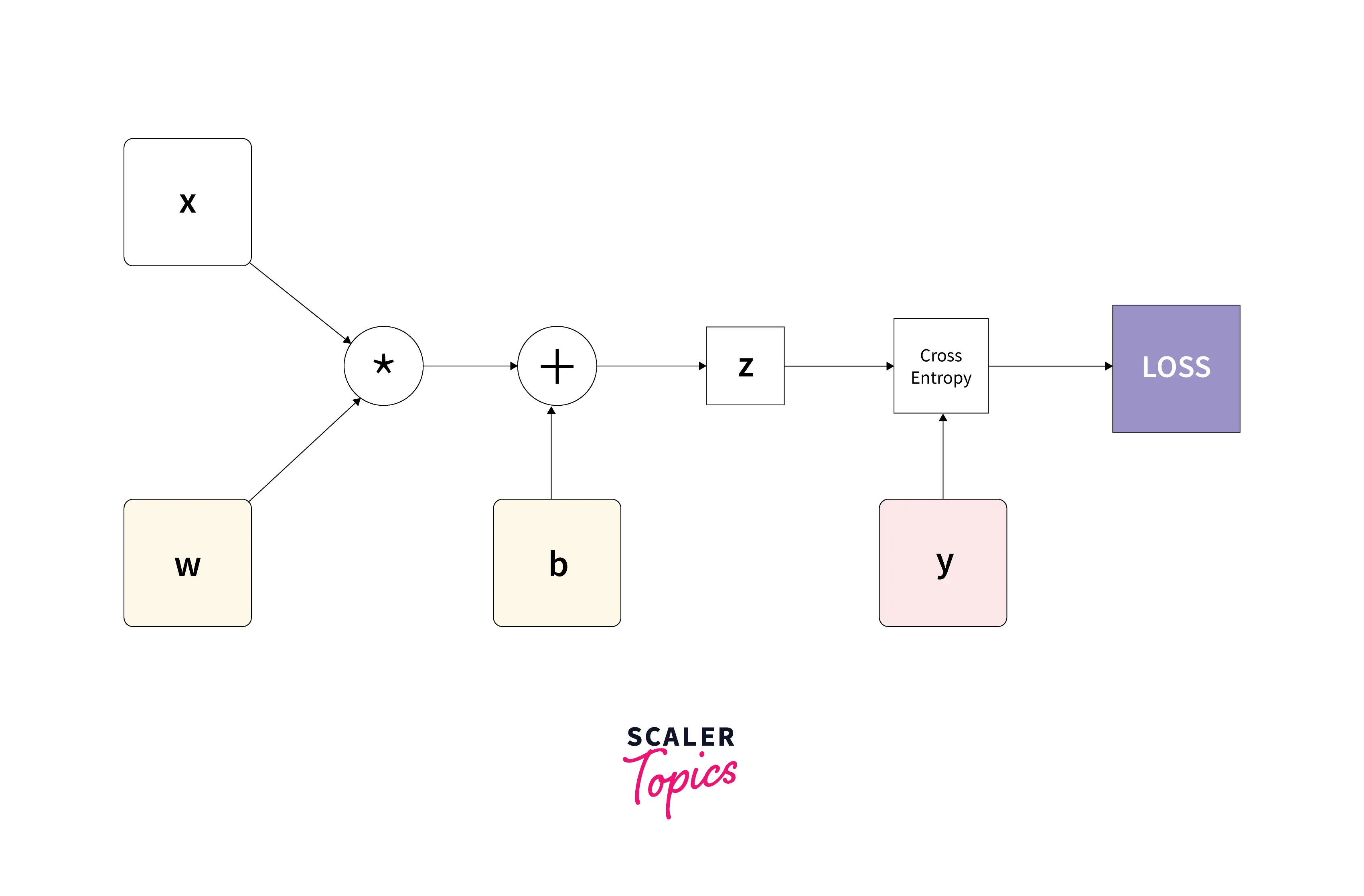
Here, the blue nodes w and b represent the parameters to be optimized, and the green node y represents the true output.

Output:

Hence, PyTorch's computational graphs are directed acyclic in nature, where the leaf nodes are the input tensors (fixed in nature) and the tensors requiring gradients (parameters of the model) while the roots are the output tensors.

Some important pointers to keep in mind while working with autograd :

1. Retaining the backward graph - After a backward call is made on a tensor, all the references to saved tensors are freed from the memory by autograd.

This is done for optimization purposes, but this also means that we cannot do a second backward call on the same tensor as now the graph has lost all the saved tensors that autograd requires to calculate the gradient.

So in the following code, as a.backward() is called a second time, PyTorch gives a runtime error telling us that the saved tensors have already been freed.

Output:

That said, there's a way we could mitigate this behavior. Using retain_graph=True causes PyTorch not to free the references to saved tensors. Hence, allowing us to backpropagate through the graph a second time. Like so-

Output:

Notice how the second backward call on tensor a ran smoothly this time without any errors. Also, notice that the gradient of a with respect to b is different after both backward calls. The next pointer explains this.

2. Accumulation of gradients - On doing a second backward call to backpropagate the gradients, PyTorch adds the values already present in the grad attribute of a tensor to the new values backpropagated a second (or maybe a third, etc.) time.

Mind here; the accumulated grad values aren't actually correct.

Why is this a problem? Clearly, while training a neural network, the accumulated gradients shall cause wrong updates to the model parameters, and hence the training will not happen in the correct way.

3. In-place operations - If a saved tensor, i.e., a tensor required for the computation of gradients, is modified in place before a backward call, autograd shall throw a run time error.

Obviously, a changed value shall cause wrong gradients to get calculated. PyTorch hence prevents wrong gradients from being calculated.

This is done by leveraging the .version attribute of tensors. Like so-

Output:

Dynamic Computation Graphs

As we've already discussed, computation graphs are essentially under the hood of automatic gradient computation by differentiation via autograd. In this section, we'll look into some more interesting details of how these computation graphs are actually built.

While computation graphs are directed acyclic in nature, they can also be of two different types - static graphs and dynamic graphs.

Pytorch uses dynamic computation graphs, and since this article is about PyTorch, we'll not go deep into a lot of details about static graphs.

But for completeness, here's what they are -

• Static Graphs - As the name suggests, static graphs are fixed, which means their structure is first defined and declared, post which values are fed to the graph in order to run it. Such graphs are hence re-used (re-fed data into) for every iteration of training, which also means that things like input size etc., need to be pre-defined. Along with the re-usability, pre-defining the graph offers a lot of scope for efficient implementation; and these two aspects make static graphs faster than dynamic ones.
• Dynamic graphs - On the other hand, dynamic graphs are defined on the go as tensors are subjected to mathematical operations. This implies that each time the graph is destroyed (that actually happens after every backward() call), new graphs are re-created from scratch. This allows for the introduction of different tensors or different operations in different iterations of training, and this also means that we can use a different input size each time.

To think about them in analogous terms, dynamic computation graphs are like dynamic memory allocation, where the memory is allocated on the heap and not allocated statically beforehand.

As for PyTorch, nodes in the graphs are the Tensors, and edges are Function objects that produce the output Tensors from input Tensors.

autograd keeps track of the complete history of the mathematical operations that lead to the formation of an output tensor by means of these dynamic graphs.

Thus, Dynamic graphs in PyTorch consist of Tensors and Function objects by means of which all computations are represented.

Let's look at how a computation graph for our simplest neural network shall look like in PyTorch -

We used torchviz to visualize our computation graph representing computations from input x all the way to the loss.

Output -

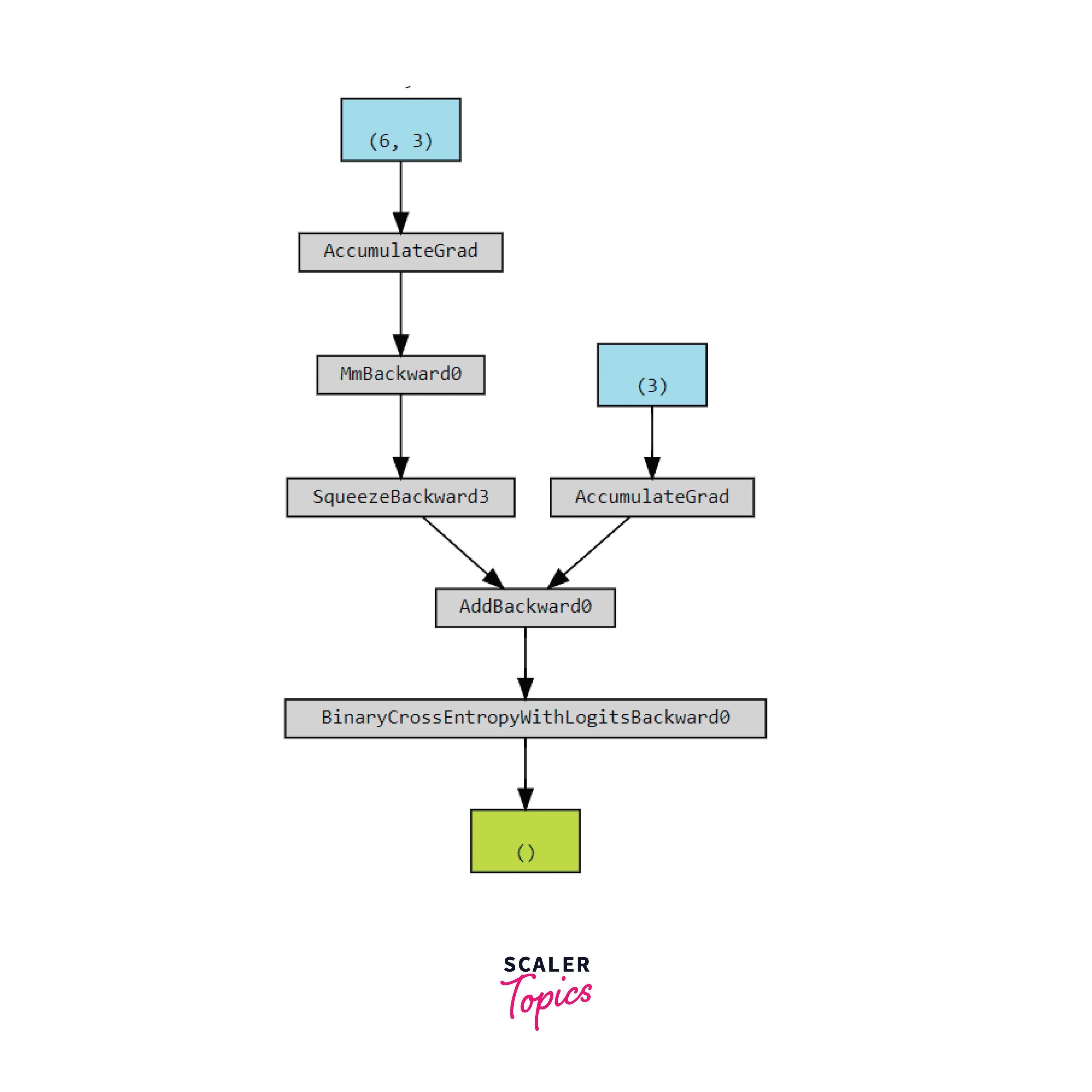
In the graph -

1. Blue nodes represent the tensors leaf tensors w (left one) and b (right one) for which the requires_grad attribute is True.
2. Gray nodes represent the function objects that are called during the backward pass and are deeped to backpropagate the gradients. Essentially, these represent the grad_fn attribute of tensors which is a reference to the function that created these tensors.
3. The green node here represents the loss tensor and is the potential starting point for the computation of gradients. It is basically the variable tensor we used to visualize the graph.

As soon as a backward call is made, this graph is backtracked, and by default, the grad attribute of the leaf tensors is populated.

Common PyTorch Modules

1. Torchvision- torchvision is a package inside Pytorch meant for the computer vision domain. It consists of Standard datasets, model architectures used for CV, and abstractions for common image transformations used to preprocess images.

It has models and training recipes available for a variety of tasks where CV is used, like image segmentation, object detection, instance segmentation, Action Classification, etc. It offers support for more than 60 pre-trained vision models that we could fine-tune or train from scratch for our use cases.

Moreover, pre-implemented /dataset loaders are available for standard datasets like ImageNet, COCO, Cityscapes, etc., which comes in handy while benchmarking new research in the domain.

2. Torchtext - torchtext is another package available inside PyTorch offering functionalities to deal with and model text data. It offers common text-preprocessing utilities and popular datasets in the field of natural language processing.

Datasets are available for a wide range of NLP tasks like Language Modeling, Sentiment Analysis, Text Classification, Question Classification, Entailment, Machine Translation, Sequence Tagging, Question Answering, and Unsupervised Learning. There are various tokenizing strategies available, like n-gram iterator, sentencepiecetokenizer, etc.

Different vocabularies are available, like that of the glove, fasttext, etc., along with support for building our own vocabulary. The most common NLP metric bleu_score is available as an abstraction and can be used as torchtext.data.metrics.bleu_score.

3. TorchAudio - Torchaudio is a companion package to PyTorch meant for audio and signal processing. It provides I/O, signal, and data processing functions, model implementations, and application components to deal with various speech operations and model audio data.

To be able to use audio data for our machine learning models, it also supports the data transformations, data augmentations, and feature extractions used for audio data.

It offers a functionality torchaudio.sox_effects.apply_effects_tensor, using which we can add sound effects to our data. TorchAudio also lets us resample audio data with ease using multiple methods by virtue of its functional and transform functionalities.

TensorFlow vs PyTorch

One hot topic of debate in the deep learning community - both academia and industry is the TensorFlow vs. PyTorch debate. While we'll not engage in any kind of debate here where one wins over the other, it's worth looking at how the two libraries potentially differ from each other.

We'll look at some key pointers to highlight the differences between the two -

• Parallelism - While both TensorFlow and PyTorch offer support for distributed training over multiple GPUs, PyTorch allows it more facilely. In a single line of code, one could wrap the model inside Pytorch's DataParallel class to enable Parallelism, while it takes writing more code to avail the same in TensorFlow.
• Deployment - No matter how shiny or accurate, a deep learning model shall be useless just sitting in a jupyter notebook. In fact, it's a waste of time and money resources if models aren't brought to life, i.e., production. When it comes to deployment, TensorFlow has been offering easy and efficient tools (TensorFlow Serving and TensorFlow Lite) for the deployment of models on cloud servers and mobile devices. While PyTorch initially lacked in this arena, it has now worked remarkably toward closing this gap by the introduction of deployment tools like TorchServe which was introduced in 2020 and supported both REST and gRPC APIs, and PyTorch Live, which supports the building of iOS and Android AI-powered apps. PyTorch live also plans to support audio and video inputs.
• Ease of use - Keras, an open-source library providing a Python API for training neural networks, was released in 2015 and became popular because of its easy-to-use nature. But, Keras didn't offer much access to low-level features and thus lacked the customizability that researchers needed to implement novel architectures. TensorFlow was released in later 2015 with the goal of solving this problem. Still, TensorFlow's non-Pythonic and somewhat difficult-to-implement nature was solved by the release of PyTorch. PyTorch, along with offering a pythonic style of coding, gives easy access to low-level features allowing for greater customizability that facilitates ease of implementation of novel architectures.

Those are the major points to differentiate the two libraries on.

Despite these listed differences, considering the fact that deep learning and hence tools used for the field have seen exponential growth in terms of development, both the libraries are essentially converging in terms of the functionality and features offered - the API experience might be quite different, nevertheless.

Where is the Pytorch Codebase?

All the code for the library is open-sourced and is available at PyTorch Github.

So, if you are an open-source enthusiast and like contributing to tools and frameworks making machine learning implementation more accessible and easier for people from varied domains, you might want to check out PyTorch GitHub to be on the lookout for potential contributions to the library.

Along, there's also this amazing discussion board called PyTorch forums that's a place to discuss and ask queries.