Ridge Regression in Machine Learning
Ridge Regression in machine learning, also known as Tikhonov regularization, is a technique used to analyze data that suffer from multicollinearity. By adding a degree of bias to the regression estimates, it reduces model complexity and prevents overfitting, resulting in more reliable and interpretable models, especially when dealing with highly correlated independent variables.
What is Ridge Regression in Machine Learning?
Ridge Regression in machine learning is a sophisticated method employed in machine learning to tackle the challenges posed by multicollinearity(a statistical phenomenon that occurs when two or more independent variables in a regression model are highly correlated with each other) among predictors within a dataset. This approach is characterized by the incorporation of L2 regularization, which directly addresses the limitations seen in ordinary least squares (OLS) regression when multicollinearity leads to high variance in model estimates, causing the predicted values to diverge significantly from the actual values.
Core Mechanism of Ridge Regression:
Ridge Regression in machine learning modifies the OLS objective by adding a penalty term to the cost function, which is proportional to the square of the magnitude of the coefficients. This penalty term aims to shrink the coefficients, thus reducing model complexity and enhancing the stability and predictability of the model. The cost function in Ridge Regression is given by:
Models of Ridge Regression
Ridge Regression extends the traditional regression model by incorporating L2 regularization to manage multicollinearity and enhance model stability. The foundational equation of any regression model, including Ridge Regression, is:
In this equation:
- represents the dependent (target) variable.
- denotes the matrix of independent (predictor) variables.
- is the vector of regression coefficients that the model aims to estimate.
- symbolizes the errors or residuals, capturing the deviation of the predicted values from the actual values.
The L2 penalty in Ridge Regression in machine learning ensures coefficients are shrunken towards zero but not eliminated. This is due to three reasons:
Continuous Shrinkage:
The penalty increases quadratically as coefficients deviate from zero, making it costly to set a coefficient exactly to zero.
Uniform Reduction:
All coefficients are reduced uniformly, ensuring no single coefficient is completely removed, which helps in managing multicollinearity without losing valuable information.
Balance Between Fit and Regularization:
The model aims to balance closely fitting the data while keeping coefficients sm
Incorporating L2 Regularization:
Ridge Regression in machine learning modifies this basic framework by adding a regularization term to the cost function used to estimate the regression coefficients. This term penalizes the size of the coefficients, effectively shrinking them towards zero but, crucially, not setting any to zero. The regularization term is controlled by the parameter (lambda), which determines the strength of the penalty applied to the size of the coefficients. The Ridge Regression cost function is thus:
Here, represents the sum of squared residuals (the difference between the observed and predicted values), and is the L2 regularization term. The parameter is key to Ridge Regression; it balances the model's fit to the data against the magnitude of the coefficients to prevent overfitting and manage multicollinearity.
Standardization using Ridge Regression
Standardization is a crucial preprocessing step in Ridge Regression, particularly due to its sensitivity to the scale of input variables. This process involves scaling the features so that they have a mean of zero and a standard deviation of one. Standardization ensures that the regularization penalty is applied uniformly across all coefficients, preventing any bias towards variables simply because of their scale.
How to Perform Standardization:
In practice, standardization is achieved by subtracting the mean of each feature and dividing by its standard deviation. For a feature , the standardized version is computed as:
where:
- is the original feature,
- is the mean of ,
- is the standard deviation of .
Bias and Variance Trade-Off
In machine learning, the concept of the bias and variance trade-off is fundamental to understanding the performance of models, including Ridge Regression. Imagine you're trying to hit a target with arrows. If your arrows consistently hit the same spot, but far from the bullseye, that's like having high bias; you're consistently wrong. If your arrows hit all over the target, you're unpredictable or have high variance. The goal is to strike the right balance, hitting the bullseye accurately and consistently.
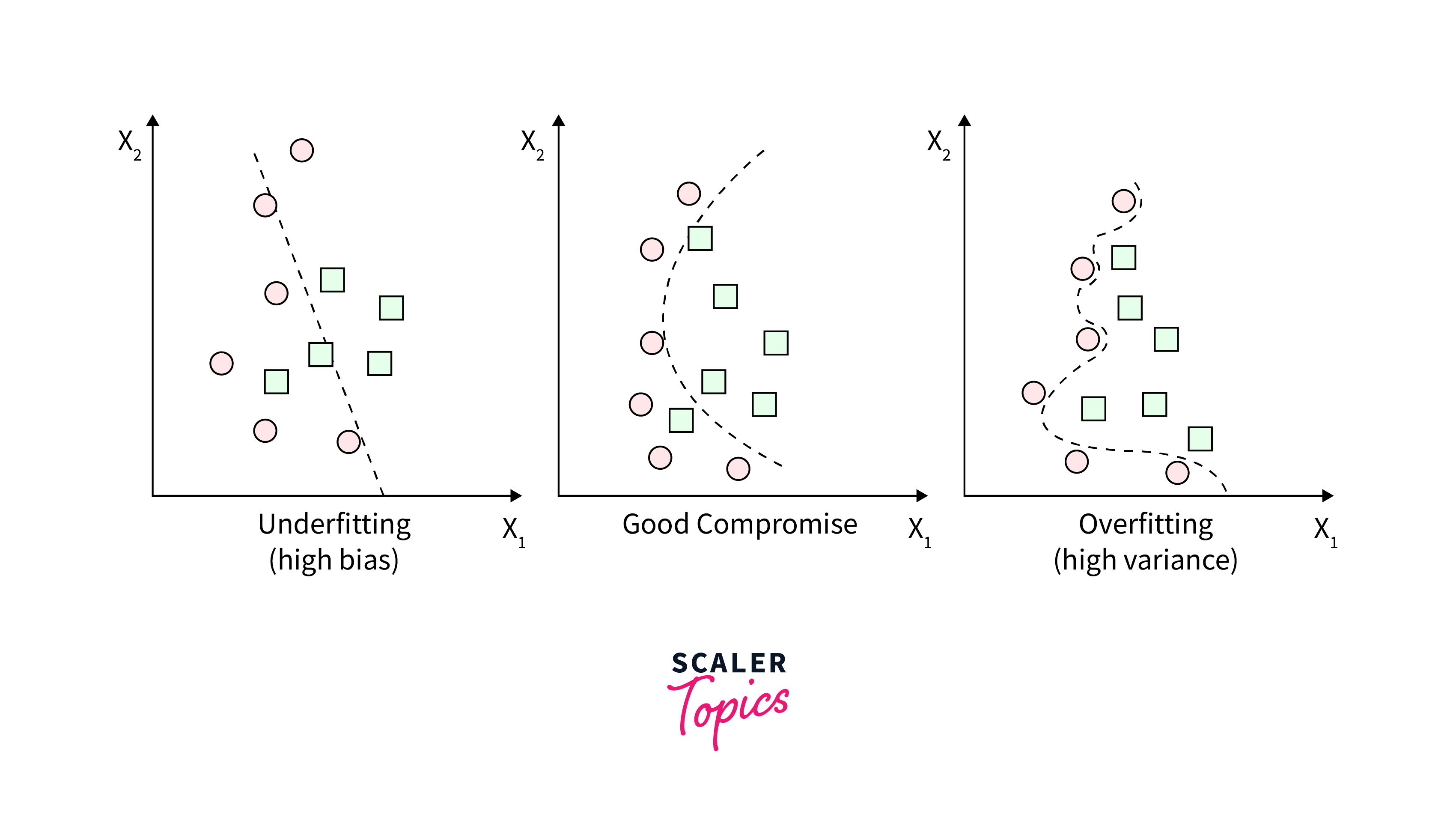
Bias:
Bias refers to the error due to overly simplistic assumptions in the learning algorithm. High bias can cause the model to miss relevant relations between features and target outputs (underfitting), akin to consistently aiming too far to the left of the target. In layman's terms, a biased model has preconceived notions that prevent it from accurately capturing the true relationship in the data.
Variance:
Variance refers to the error due to too much complexity in the learning algorithm. High variance can cause the model to model the random noise in the training data (overfitting), like adjusting your aim for each shot based on the last one you took, resulting in shots scattered all over the place. A model with high variance pays too much attention to the training data, losing the ability to generalize from the model to new data.
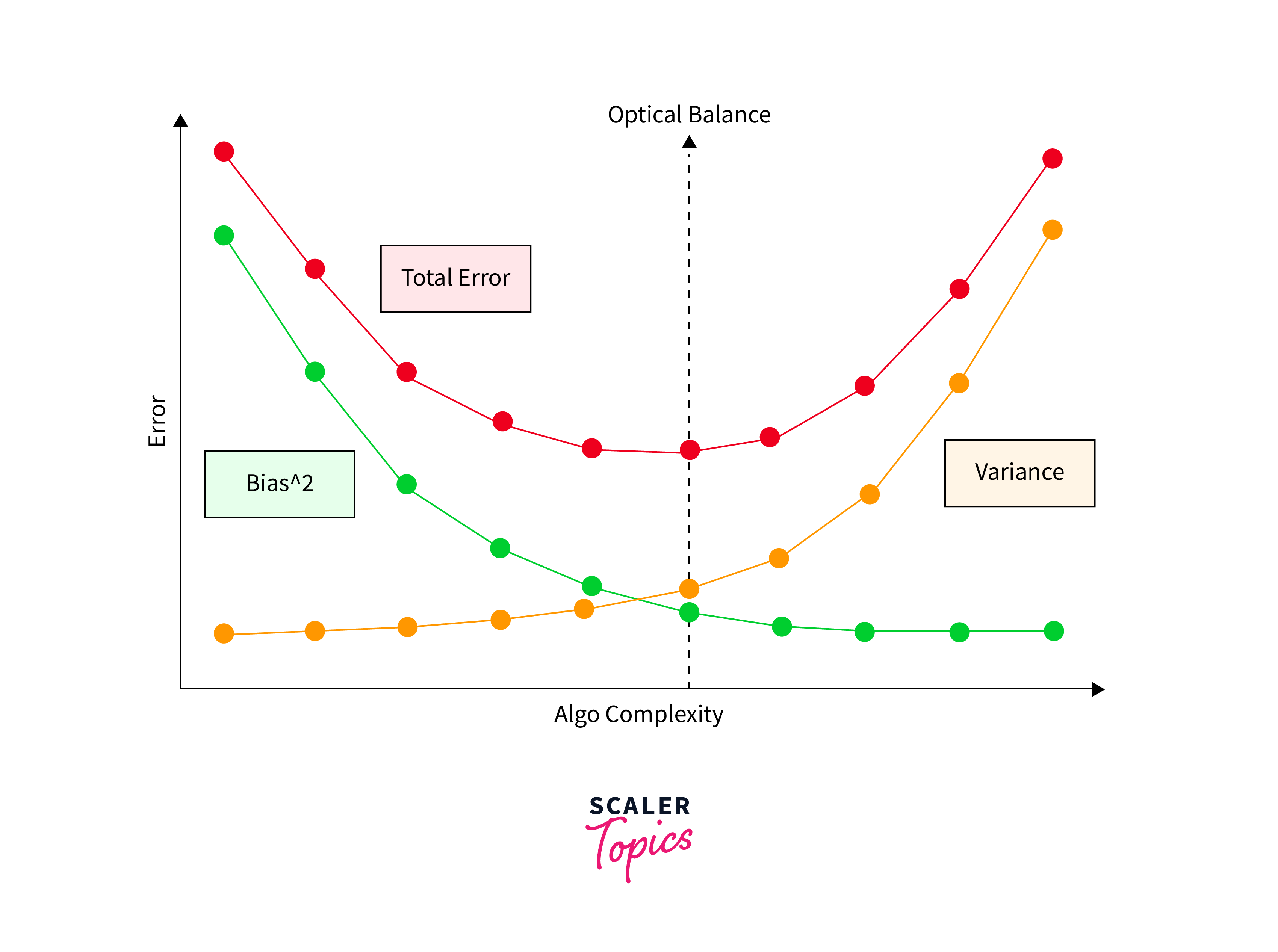
The Trade-Off:
The trade-off is a balancing act between bias and variance. Ideally, you want a model that accurately captures the underlying patterns in the data (low bias) and generalizes well to new, unseen data (low variance). However, reducing bias often increases variance, and vice versa. Imagine trying to adjust your aim to hit the bullseye (reducing bias) without getting your shots too scattered (increasing variance).
Ridge Regression's Role:
Ridge Regression helps in this balancing act by adding a penalty on the size of coefficients. This penalty term discourages fitting the model too closely to the training data, which can reduce variance (making your shots less scattered) but might increase bias (your average shot might be further from the bullseye). The regularization parameter () in Ridge Regression controls this balance: a higher increases bias and reduces variance, while a lower reduces bias and increases variance.
Ridge Regression in Machine Learning: Assumptions
Ridge Regression requires scaled variables, a linear relationship between predictors and the target, and operates best when data is divided into training and testing sets for model evaluation, facilitated by essential computational libraries.
Key Assumptions in Ridge Regression:
- Linearity:
The relationship between predictors and the target variable should be linear. - Multivariate Normality:
The residuals (errors) of the model should be normally distributed. - No Multicollinearity (Or Less Concerned):
Although Ridge Regression is used to mitigate multicollinearity, the basic assumption still favors minimal correlation between independent variables. - Homoscedasticity:
The variance of error terms should be constant across all levels of the independent variables. - Independence:
Observations should be independent of each other.
When to Use Ridge Regression?
Ridge Regression is particularly useful in situations where you're dealing with data that has a high degree of multicollinearity—meaning the independent variables (predictors) are highly correlated with each other. This condition can cause issues in traditional linear regression models, such as inflated variances of the estimated coefficients, leading to unreliable and unstable predictions.
Scenarios ideal for Ridge Regression:
Ridge Regression is ideal for scenarios with high multicollinearity, as it stabilizes estimates through a penalty term. It's useful when there are more predictors than observations by allowing coefficient estimation via regularization. This method also prevents overfitting by shrinking coefficients to enhance model generalizability and applies regularization to improve prediction accuracy by controlling model complexity.
Implementing Ridge Regression using Python
Step 1: Import Necessary Libraries
First, you'll need to import the libraries required for the data manipulation, model fitting, and evaluation:
Step 2: Load and Prepare Your Data
Load your dataset and prepare it for modeling. This preparation typically involves splitting your data into features (X) and the target variable (y), followed by a train-test split:
Step 3: Standardize the Features
Since Ridge Regression is sensitive to the scale of input variables, it's a good practice to standardize the features:
Step 4: Fit the Ridge Regression Model
Initialize the Ridge Regression model, specifying the regularization strength (alpha). Then, fit the model to your scaled training data:
Step 5: Make Predictions and Evaluate the Model
Use the trained model to make predictions on the test set, and evaluate the model's performance using an appropriate metric, such as the mean squared error (MSE):
Output:-
Lasso Regression vs. ridge Regression
| Feature | Lasso Regression | Ridge Regression |
|---|---|---|
| Penalty Type | L1 regularization (penalizes the absolute value of coefficients). | L2 regularization (penalizes the square of the coefficients). |
| Coefficient Shrinkage | Can shrink some coefficients to exactly zero. | Shrinks coefficients towards zero but not to zero. |
| Feature Selection | Can perform automatic feature selection by eliminating variables. | Does not perform automatic feature selection. |
| Model Complexity | Tends to produce simpler models with fewer variables. | Tends to produce models that include all variables, albeit with smaller coefficients. |
| Solution Path | Non-linear and piecewise linear, leading to sparse solutions. | Smooth and continuous, which does not naturally lead to sparsity. |
| Multicollinearity | Effective in handling multicollinearity by excluding irrelevant predictors. | Manages multicollinearity by distributing the effect across all predictors. |
FAQs
Q. Can Lasso and Ridge Regression be used together?
A. Yes, combining Lasso and Ridge Regression techniques is known as Elastic Net, which incorporates both L1 and L2 regularization to leverage the benefits of both methods.
Q. When should I prefer Ridge Regression over Lasso Regression?
A. Prefer Ridge Regression when you have multicollinearity among variables and you want to include all features in the model without excluding any, as it shrinks coefficients evenly without setting them to zero.
Q. Is Lasso Regression better for feature selection?
A. Yes, Lasso Regression is often preferred for feature selection because it can shrink some coefficients to zero, effectively removing those variables from the model.
Q. How does the choice of alpha affect Lasso and Ridge Regression models?
A. The alpha parameter controls the strength of the regularization. In both models, a higher alpha value increases the penalty on the coefficients, leading to simpler models. The optimal alpha balances model complexity with prediction accuracy and is typically found through cross-validation.
Conclusion
- Ridge Regression provides a solution to overfitting and multicollinearity through L2 regularization, applying a uniform effect across all variables to maintain model stability without excluding any features.
- In scenarios with high multicollinearity among predictors, Ridge Regression ensures stability by distributing the regularization effect uniformly, thus retaining all predictors with smaller coefficients.
- Elastic Net offers a hybrid solution that incorporates the multicollinearity management of Ridge, allowing for a balanced approach to regression modeling that addresses both overfitting and feature selection.