Excel SUMIFS Function

What is the SUMIFS Formula in Excel?

The SUMIFS formula in Excel is a powerful function used to calculate the sum of values that meet multiple specified criteria points. It enables you to perform advanced data analysis and aggregation tasks with ease. The formula has a straightforward syntax, making it user-friendly for both beginners and experienced Excel users.

SUMIFS Formula in Excel Syntax

The SUMIFS function in Excel is used to calculate the sum of values in a range based on multiple criteria. Its syntax is as follows:

SUMIFS Formula in Excel Arguments

The SUMIFS function in Excel allows you to sum values based on multiple criteria. To use it effectively, you need to understand the various arguments it accepts. Let's delve into the details of each argument:

1. sum_range (required)
2. criteria_range1 (required)
3. criteria1 (required)
4. [criteria_range2, criteria2], [criteria_range3, criteria3], ... (optional)

SUMIFS Formula in Excel Return Value

The SUMIFS formula in Excel returns the sum of values from a specified sum_range that meets all the specified criteria. This returned value is the result of adding up all the values in the sum_range that satisfy all the conditions set in the formula.

For example, if you have a dataset with sales figures in column B, product names in column A, and regions in column C, and you use the SUMIFS formula like this:

SUMIFS Formula in Excel Examples

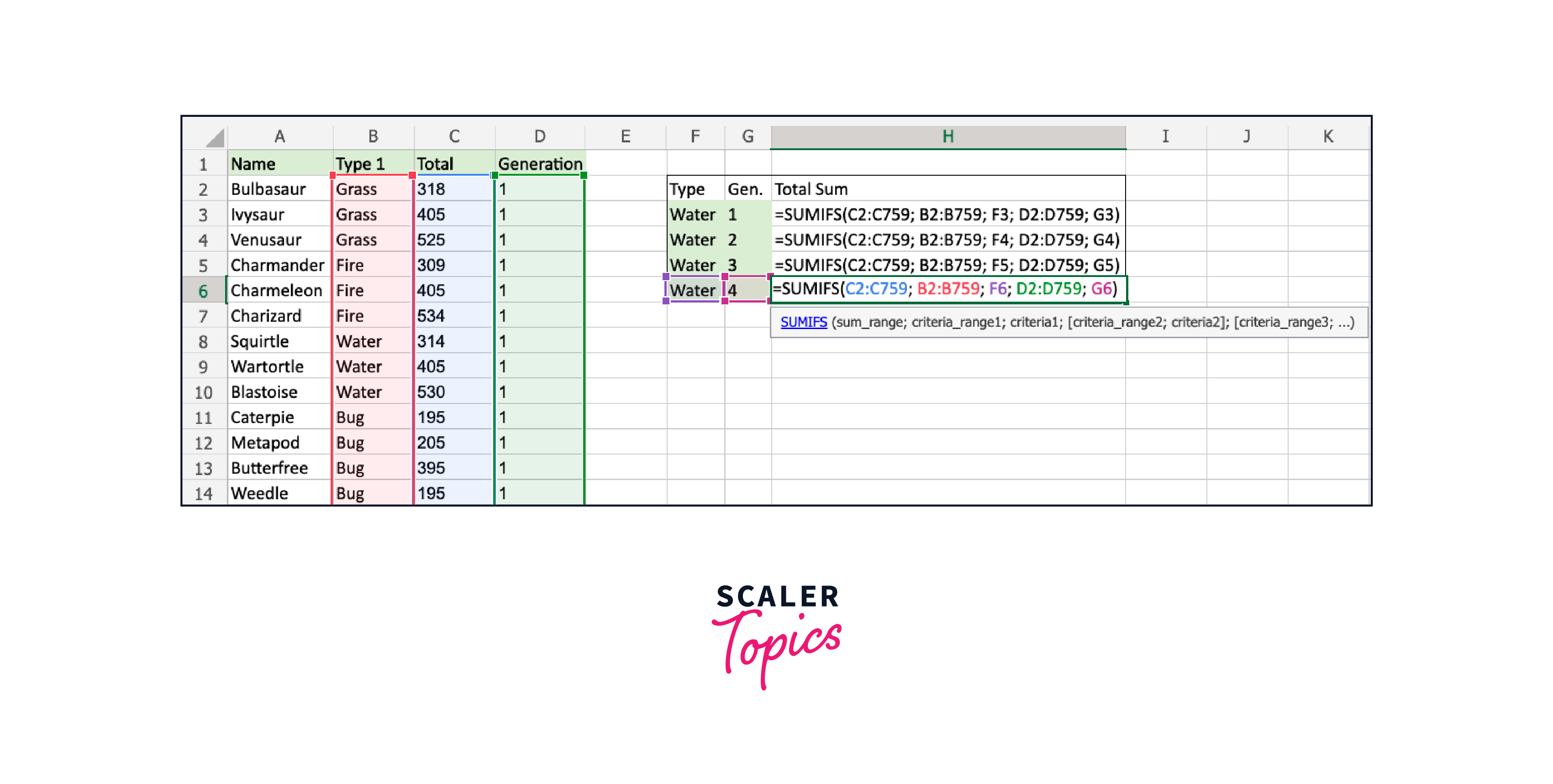
How to Use SUMIFS in Excel (AND Logic)?

In Excel, you can use the SUMIFS function with AND logic to sum values that meet multiple criteria simultaneously. When you use AND logic, all the specified conditions must be true for a cell to be included in the sum. Here's how to use SUMIFS with AND logic:

1. Syntax of SUMIFS with AND logic:

The syntax for SUMIFS with AND logic is as follows:

• sum_range:
  This is the range of cells containing the values you want to sum based on the specified criteria.
• criteria_range1, criteria1:
  These are the first criteria range and its corresponding criteria.
• You can add more pairs of criteria_range and criteria for additional criteria.

2. Enter the Formula:

Let's say you have a dataset with sales figures in column B, product names in column A, and regions in column C. If you want to calculate the total sales for "Apples" in the "East" region, you would use the following formula:

• B2:B10 is the sum_range (sales figures).
• A2:A10 is the first criteria_range (product names).
• "Apples" is the first criterion, specifying that you want to sum sales for the product "Apples".
• C2:C10 is the second criteria_range (regions).
• "East" is the second criterion, specifying that you want to sum sales in the "East" region.

3. Press Enter:

After entering the formula, press the Enter key. Excel will calculate and display the total sales for "Apples" in the "East" region in the cell where you entered the formula.

Excel SUMIF with Multiple Criteria (OR Logic)

SUMIF with Multiple OR Criteria (Using SUM Function):

Suppose you have a dataset with sales figures in column B, and you want to sum the sales for "Apples" or "Bananas" products. You can use the following formula:

• A2:A10 is the range where you have the product names.
• {"Apples", "Bananas"} is an array of criteria, specifying the products you want to sum.
• B2:B10 is the sum_range, containing the sales figures.

This formula first applies the SUMIF function to each criterion separately and then sums the results, effectively applying OR logic.

Excel SUMIFS with Multiple OR Conditions

Suppose you have a dataset with sales figures in column B, product names in column A, and regions in column C, and you want to sum the sales for "Apples" or "Bananas" products in either the "North" or "East" regions. You can use the following formula:

Using SUM in Array Formulas

To use the SUM function in an array formula, follow these steps:

1. Select the Range:

Start by selecting the range of cells where you want the result of the array formula to appear.

2. Enter the Formula:

Type your array formula directly into the formula bar. Array formulas are enclosed in curly braces {}. You don't need to type these braces manually; Excel adds them automatically when you press Ctrl+Shift+Enter after entering the formula.

For example, let's say you have values in cells A1 to A5 and you want to sum them using an array formula. Enter the following formula:

However, instead of just pressing Enter, you should press Ctrl+Shift+Enter. Excel will then add the curly braces and calculate the sum of the selected range.

3. View the Result:

After pressing Ctrl+Shift+Enter, Excel will display the result of the array formula in the selected range. The formula will now appear within curly braces, indicating that it's an array formula.