R Survival Analysis

Survival Analysis in R Programming Language

Survival analysis in the R programming language offers a robust framework for analyzing time-to-event data. With R's extensive libraries and packages, conducting survival analysis becomes both accessible and powerful.

For instance, in a clinical study monitoring disease recurrence after treatment, survival analysis is essential as it considers the censored nature of the data and provides estimates of the probability of disease recurrence over time. Traditional statistical methods are ill-suited for such data, making survival analysis a requisite tool for extracting valuable insights from time-to-event datasets.

• Kaplan-Meier Estimator: One fundamental method in survival analysis in R is the Kaplan-Meier estimator. It allows us to estimate survival probabilities over time, especially when dealing with censored data, where not all events have occurred by the study's end. This method is a crucial step in understanding how survival rates change over time.
• Cox Proportional Hazards Model: R provides a comprehensive platform for fitting the Cox Proportional Hazards Model. This model enables researchers to assess the impact of multiple covariates on the hazard rate, quantifying how various factors affect the risk of experiencing the event. It's a powerful tool for identifying significant predictors in survival analysis.

Kaplan-Meier Estimator and Survival Curves

In survival analysis in R, one of the fundamental tools you'll frequently encounter is the Kaplan-Meier estimator. This method helps estimate the probability of an event occurring at different time points. It's particularly useful when dealing with time-to-event data, where not all events may have occurred by the end of the study, resulting in censored data.

Formula:

Where:

• S(t) represents the estimated survival probability at time t .
• ti are the distinct event times in your dataset.
• di denotes the number of events occurring at time ti.
• ni represents the number of individuals at risk (i.e., still in the study) just before time ti.

Example:

Let's say we have a dataset of patients in a clinical trial, and we want to estimate the survival probability of these patients over time. Here's a step-by-step example of how you can do this in R:

In this dataset:

• time represents the time variable, which signifies the duration (in months, for instance) until a specific event occurs.
• event is a binary variable. It takes the value of 1 if the event of interest occurred within the given time frame and 0 if it did not. In a clinical trial, 'event' might indicate whether a patient experienced the expected outcome (e.g., disease recurrence) during the observation period (specified in 'time').

Output:

In this example, we first load the survival package. Then, we create a dataset with time representing the time to the event and 'event' indicating whether the event occurred (1) or not (0). We use the survfit() function to fit the Kaplan-Meier estimator to this data.

Let's interpret the output:

• n: This indicates the total number of individuals (patients) in the dataset, which is 5 in this case.
• events: It represents the number of events that have occurred during the study period. In this dataset, 3 events occurred (e.g., patients experienced the event of interest, such as disease recurrence).
• median: The median survival time is estimated to be 48 units (e.g., months). This means that, on average, half of the patients in the study experienced the event of interest by 48 months.
• 0.95LCL (Lower Confidence Limit) and 0.95UCL (Upper Confidence Limit): These values indicate the lower and upper bounds of the 95% confidence interval for the median survival time. In this case, the lower confidence limit is 24, but the upper confidence limit is not available (NA).

Cox Proportional Hazards Model

In the realm of survival analysis in R, the Cox Proportional Hazards Model is a powerful tool that helps us understand how various factors influence the risk (hazard) of an event occurring over time. This model is particularly useful when you want to explore the impact of multiple covariates on survival probabilities.

Example:

Suppose we have a dataset of cancer patients, and we want to investigate how age, gender, and treatment type influence the hazard of cancer recurrence. Here's a step-by-step example of how to use the Cox Proportional Hazards Model in R:

Output:

In this example, we load the survival package and create a dataset containing covariates (age, gender, and treatment) along with survival data (time and event). We then use the coxph() function to fit the Cox Proportional Hazards Model to the data.

Here's a concise interpretation:

• The model results indicate that age and genderMale do not have statistically significant effects on the hazard of the event, as their p-values are above the typical significance level of 0.05.
• The treatmentB variable is flagged with NA coefficients, suggesting a potential issue with this variable, such as perfect separation in the data, which needs further investigation and data adjustment.
• The concordance value of 0.6 indicates moderate predictiveness of the model in terms of event ordering, but none of the hypothesis tests (Likelihood ratio, Wald, Score) show significant associations between the covariates and survival.

Fitting Survival Models in R

In survival analysis in R, fitting survival models is a fundamental step to glean insights from your data. This process involves package installation, understanding the syntax, and applying these models to real-world data.

Package Installation:

Before fitting survival models in R, you need to install the survival package, which provides essential functions for survival analysis:

Once installed, you can load the package for use in your R session:

Syntax:

To fit survival models in R, you'll primarily use the coxph() function for the Cox Proportional Hazards Model. Here's the basic syntax:

• Surv(time, event) specifies the survival object, where time is the time-to-event variable, and 'event' indicates whether the event occurred (1) or not (0).
• covariate1 + covariate2 + ... represents the covariates you want to include in your model.
• data = your_data is the dataset you are using for analysis.

Example:

Let's work through an example of fitting a Cox Proportional Hazards Model for survival analysis in R using a hypothetical dataset of cancer patients. We want to investigate how age, gender, and treatment type influence survival:

Output:

Applying surv() and survfit()

In survival analysis in R, two essential functions that allow you to manipulate and visualize time-to-event data are surv() and survfit(). These functions are invaluable for creating survival objects, estimating survival probabilities, and generating survival curves.

surv() Function:

The surv() function is used to create a survival object, which is a fundamental data structure in survival analysis. This function takes two arguments:

• Time-to-event data: This is typically represented as a formula using the Surv() function. For example, Surv(time, event) indicates that 'time' is the time-to-event variable, and 'event' indicates whether the event occurred (1) or not (0).
• Data: The dataset you are working with.

Example:

Here's an example of how to use the surv() function to create a survival object:

In this example, we load the survival package, and then we create a survival object using the surv() function. The formula Surv(time, event) ~ 1 specifies that we are using time and event as the time-to-event data.

survfit() Function:

The survfit() function is used to estimate survival probabilities and generate survival curves based on the survival object created with surv(). It provides a visual representation of how survival probabilities change over time.

Example:

Continuing from the previous example, here's how to use the survfit() function to estimate survival probabilities and create a survival curve:

Applying surv() and survfit() function

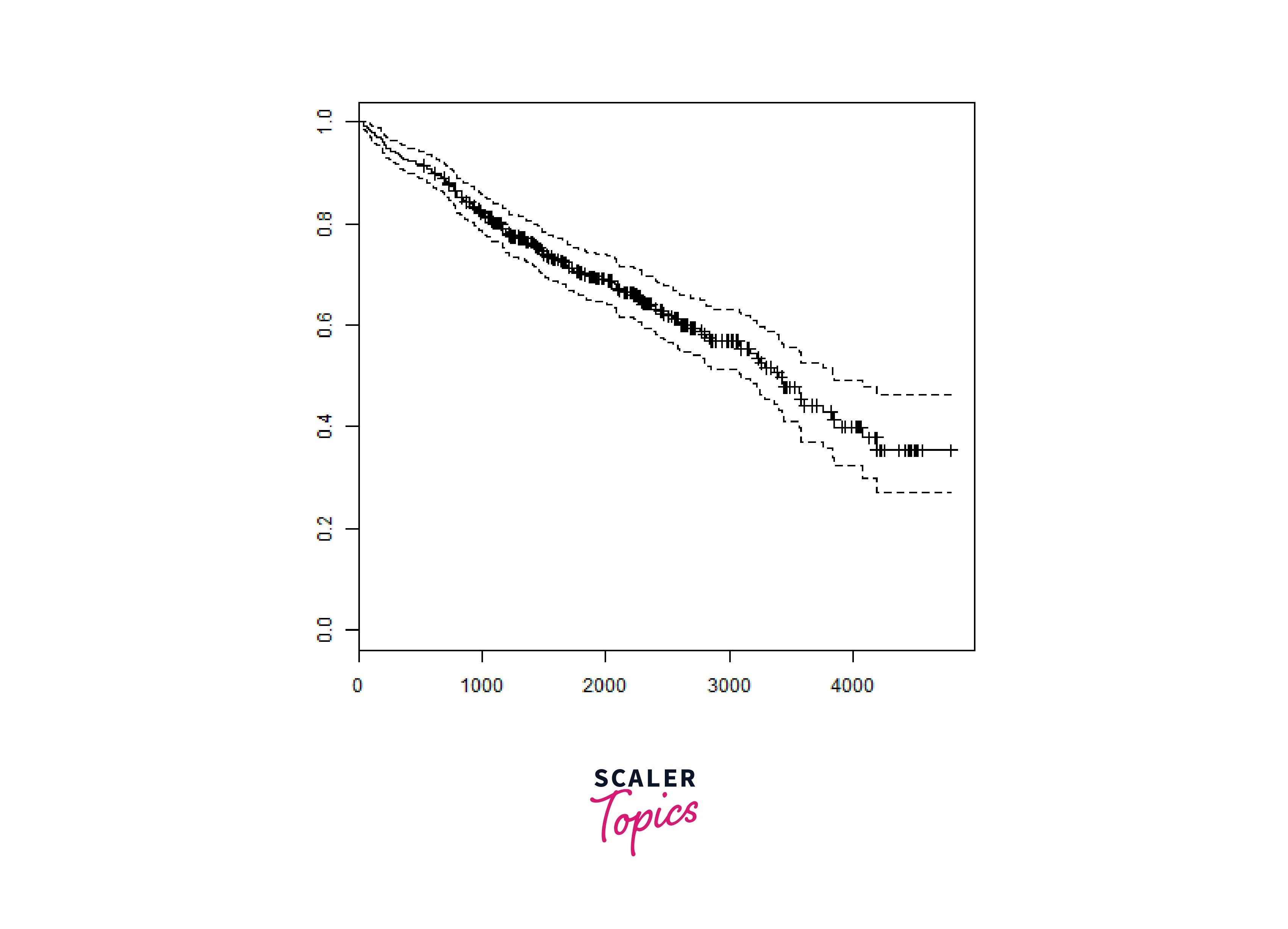
We will consider the data set named "pbc" present in the survival packages installed above. It describes the survival data points about people affected with primary biliary cirrhosis (PBC) of the liver. Among the many columns present in the data set we are primarily concerned with the fields "time" and "status". Time represents the number of days between registration of the patient and earlier of the event between the patient receiving a liver transplant or death of the patient.

Output:

Now we proceed to apply the Surv() function to the above data set and create a plot that will show the trend.

Output: