K-Nearest Neighbor (KNN) Algorithm in Machine Learning

Overview
KNN is a reasonably simple classification technique that identifies the class in which a sample belongs by measuring its similarity with other nearby points.
Though it is elementary to understand, it is a powerful technique for identifying the class of an unknown sample point.
In this article, we will cover theKNN Algorithm in Machine Learning, how it works, its advantages and disadvantages, applications, etc., in detail. We will also present a python code for the KNN Algorithm in Machine Learning for a better understanding of readers.
Additionally, we highly recommend our comprehensive machine learning course, which covers a wide range of topics, including the KNN Algorithm, to help readers deepen their understanding and practical skills in this field.
Let's get started
Introduction to KNN Algorithm in Machine Learning
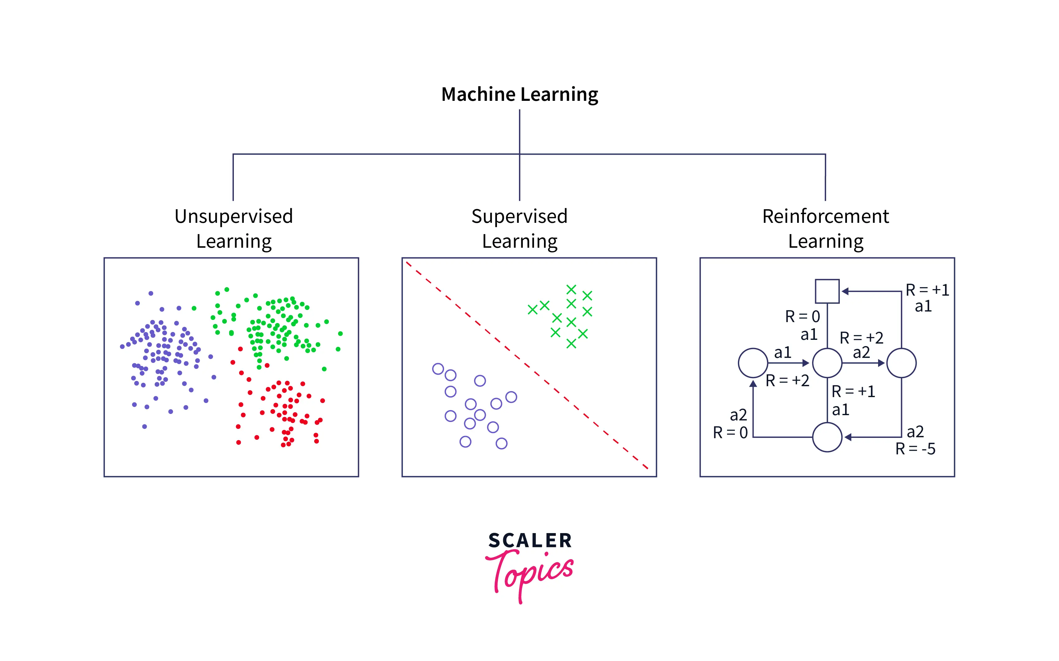
There are three main subsets of Machine Learning:
Supervised Learning, Unsupervised Learning, and Reinforcement Learning.
Stop learning AI in fragments—master a structured AI Engineering Course with hands-on GenAI systems with IIT Roorkee CEC Certification
AI Engineering Course Advanced Certification by IIT-Roorkee CEC
A hands on AI engineering program covering Machine Learning, Generative AI, and LLMs - designed for working professionals & delivered by IIT Roorkee in collaboration with Scaler.
Enrol Now
In unsupervised learning, we try to solve a problem that does not utilize past data. For example, given a scatter plot, our task is to find relevant clusters and group the data accordingly.
In reinforcement learning, we define a set of favorable outcomes and a set of unfavorable outcomes. Then the algorithm is allowed to explore the problem space. If it achieves a favorable outcome, it tries to repeat the actions that led to it, and if it achieves an unfavorable outcome, it tries to avoid the actions that led to it.
In supervised learning, you are given a set of inputs and a set of correct outputs.
Using this supervisory data, you need to write an algorithm that learns the patterns from these input-output mappings so that the next time when you get a fresh input, you can accurately estimate its corresponding output. Given the areas of many neighboring houses (in square feet), and their prices, we can predict the price of a new house.
Given the biological parameters of many tumors (cell size, cell shape, etc.) and whether they are benign or malignant, we can predict the behavior of a new, unknown tumor. This specific example is called a Classification Problem, which is what KNN solves.
It is important to note that the type of learning does not depend on which one looks better or has better accuracy but instead on the nature of the problem.
How does K-Nearest Neighbours Work?
The steps for the KNN Algorithm in Machine Learning are as follows:
- Step - 1 :
Select the number K of the neighbors - Step - 2 :
Calculate the Euclidean distance of each point from the target point. - Step - 3 :
Take the K nearest neighbors per the calculated Euclidean distance. - Step - 4 :
Among these k neighbors, count the number of the data points in each category. - Step - 5 :
Assign the new data points to that category for which the number of neighbors is maximum.
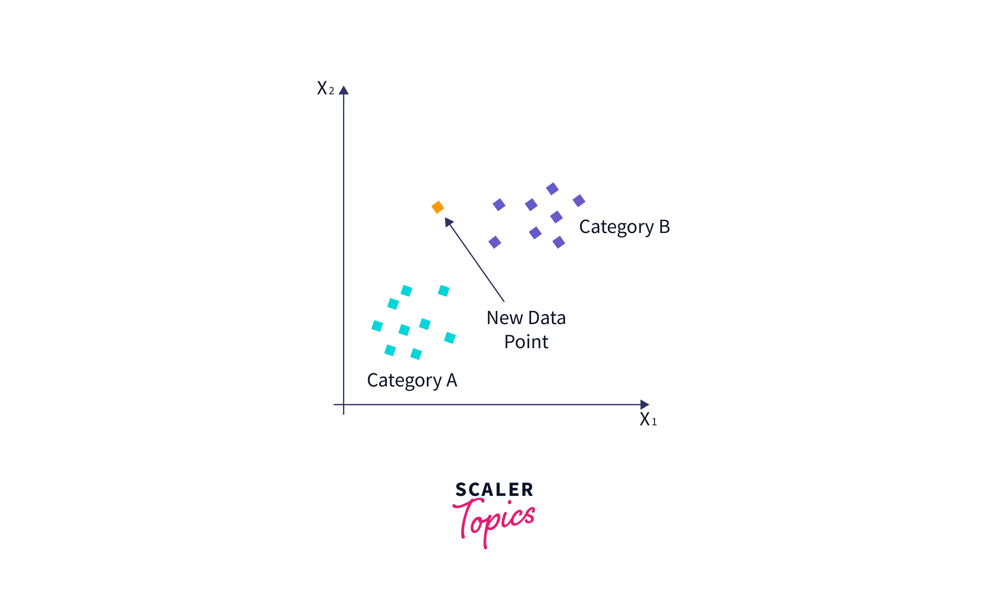
Suppose we have a new data point and need to put it in the required category. Consider the below image :
Master structured AI Engineering + GenAI hands-on, earn IIT Roorkee CEC Certification at ₹40,000
AI Engineering Course Advanced Certification by IIT-Roorkee CEC
A hands on AI engineering program covering Machine Learning, Generative AI, and LLMs - designed for working professionals & delivered by IIT Roorkee in collaboration with Scaler.
Enrol Now- First, we will choose the number of neighbors as k=5.
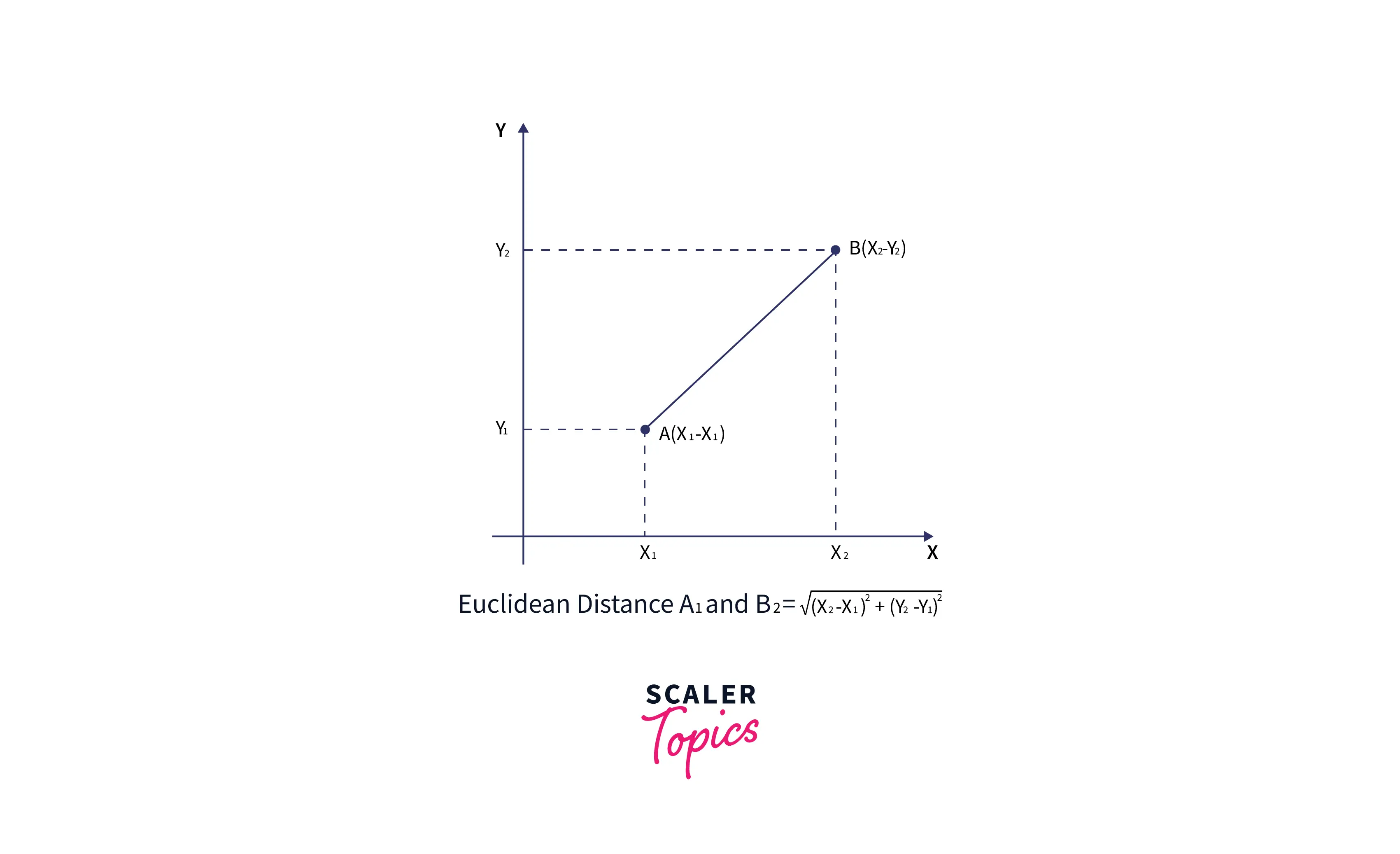
- Next, we will calculate the Euclidean distance between the data points. The Euclidean distance is the distance between two points, which we have already studied in geometry. It can be calculated as :
- By calculating the Euclidean distance, we got the nearest neighbors, as three nearest neighbors in category A and two nearest neighbors in category B. Consider the below image :
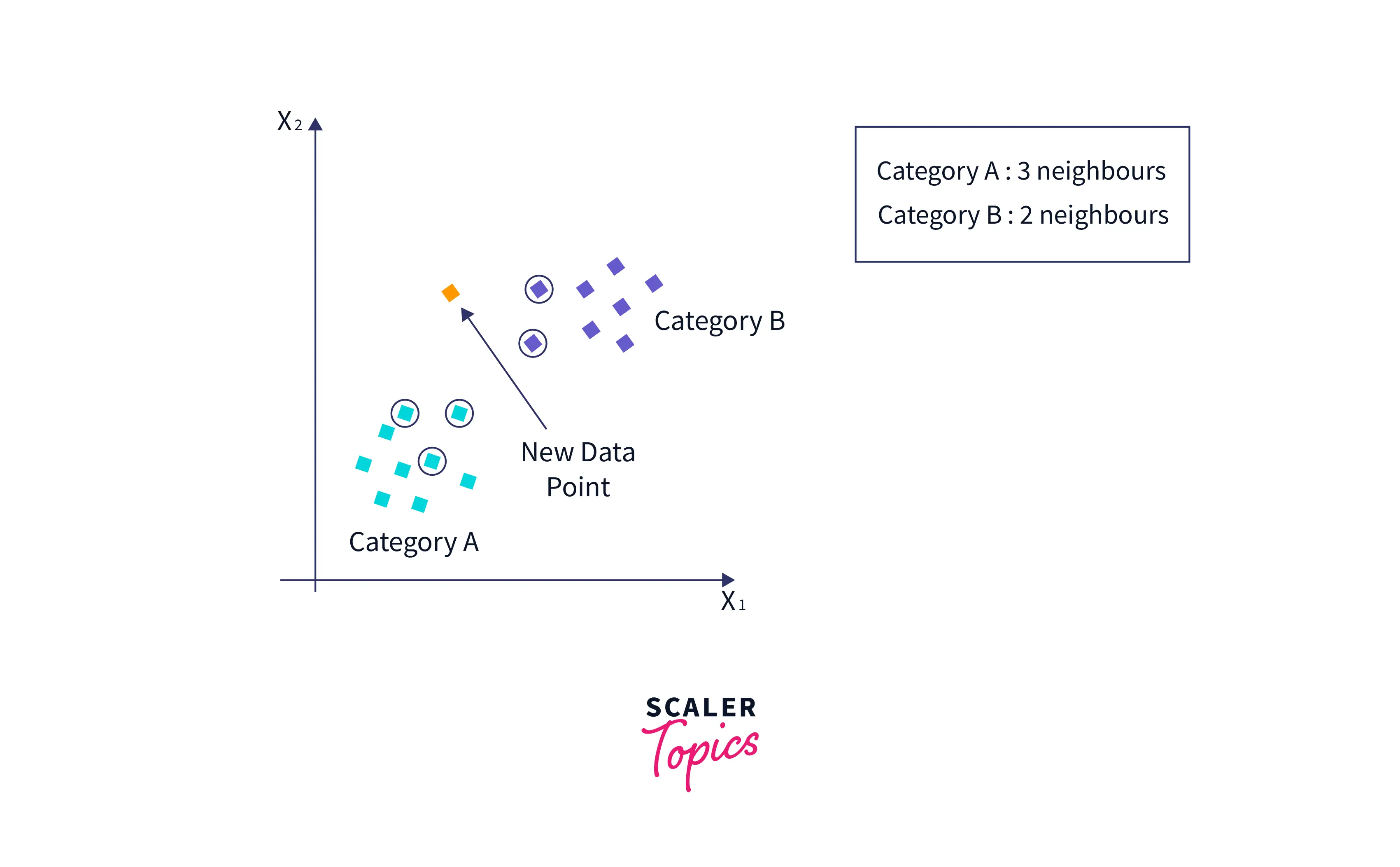
- As we can see, the three nearest neighbors are from category A. Hence this new data point must belong to category A.
Transform Your Career
Choose from our industry-leading programs designed for career success
Modern Software and AI Engineering Program
Master full-stack development with AI integration

Modern Data Science and ML with specialisation in AI
Advanced data science techniques with AI specialization
Advanced AIML with Specialisation in Agentic AI
Deep dive into AIML with focus on Agentic systems
DevOps, Cloud & AI Platform Engineering
Build and manage AI-powered cloud infrastructure
AI Engineering Advanced Certification by IIT-Roorkee
Premier AI engineering certification from IIT-Roorkee
Why do we Need K-Nearest Neighbours Algorithm?
K Nearest Neighbor is one of the fundamental algorithms in machine learning. Machine learning models use a set of input values to predict output values. KNN is one of the simplest forms of machine learning algorithms mostly used for classification. It classifies the data point on how its neighbor is classified.
KNN classifies the new data points based on the similarity measure of the earlier stored data points. For example, if we have a dataset of tomatoes and bananas. KNN will keep similar criteria like shape and color. Then, when a new object comes, it will check its similarity with the color (red or yellow) and shape.
How to Determine the K Value ?
Choosing an appropriate value of k in KNN is crucial to get the best out of the model. If the value of K is small, the model's error rate will be large, especially for new data points, since the number of votes is small. Hence, the model is overfitted and highly sensitive to noise in the input. Moreover, the boundaries for classification become too rigid, as seen in the image below.
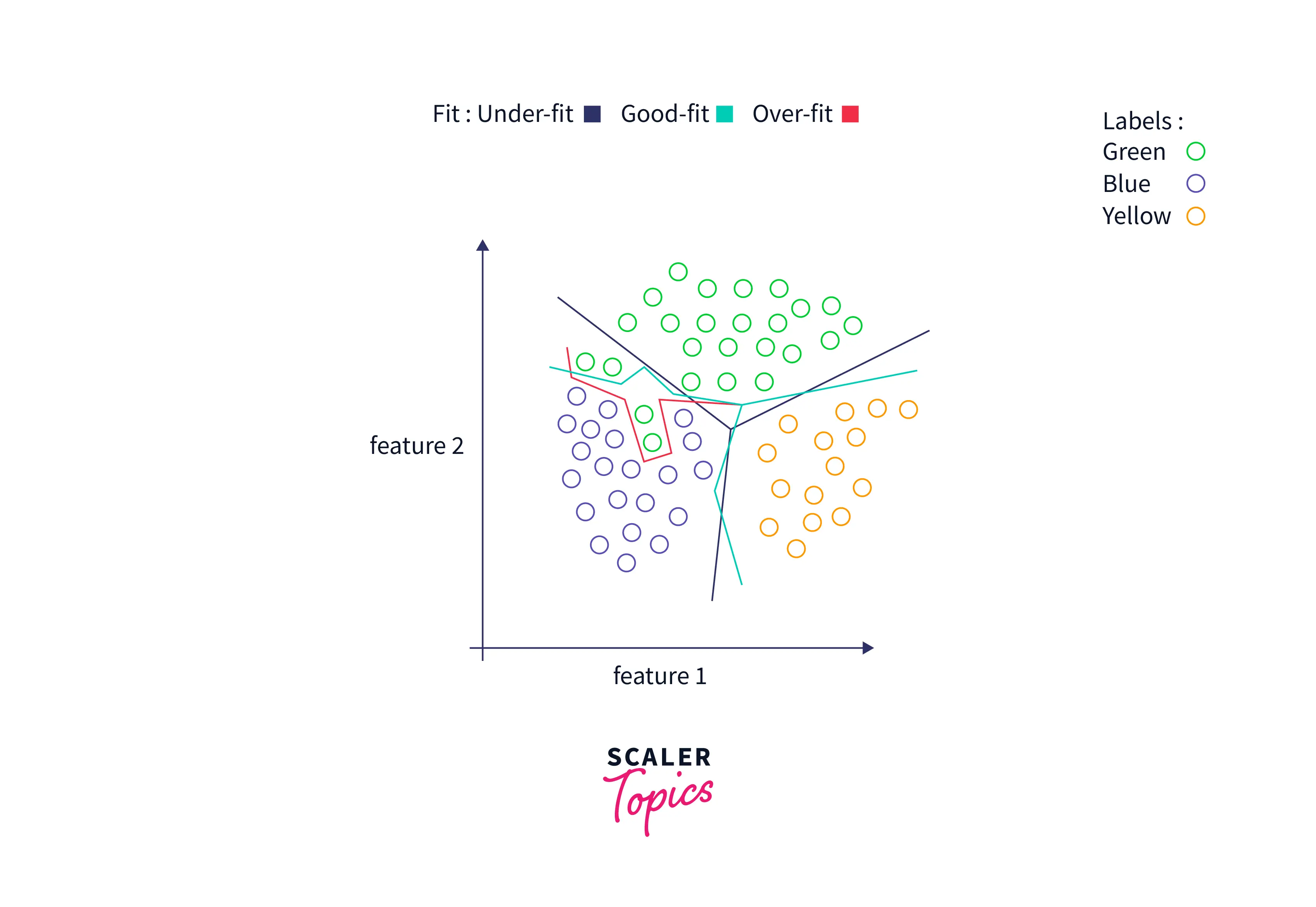 On the other hand, if the value of K is large, the model's boundaries become loose, and the number of misclassifications increases. In this case, the model is said to be underfitted.
There is no fixed method to find k, but the following points might help :
-
Set K as an odd number, so we have an extra point to settle tie-breakers in extreme cases.
-
A decent value of k can be the square root of the number of data points involved in the training dataset. Of course, this method may not work in all cases.
-
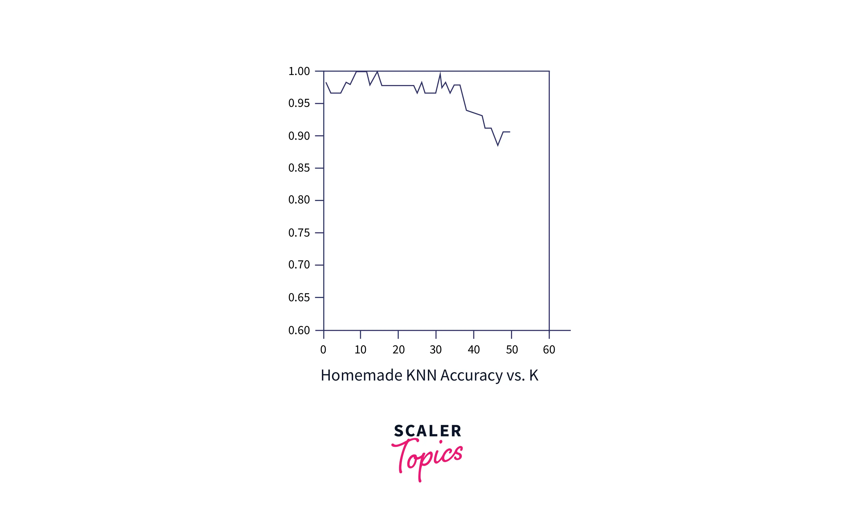
Plot the error rate vs. K graph :
First, split the supervisory dataset into two categories:
- Training and
- Testing data.
The training data should be more than the latter. Start with k = 1 and predict with KNN for each data point in the testing data. Compare these predictions with the actual labels, and find the model's accuracy. Find the error rate.
Repeat this process for different values of k and plot the error rate vs. k graph, and choose the value of k which has the least error rate.
Become the Ai engineer who can design, build, and iterate real AI products, not just demos with an IIT Roorkee CEC Certification
AI Engineering Course Advanced Certification by IIT-Roorkee CEC
A hands on AI engineering program covering Machine Learning, Generative AI, and LLMs - designed for working professionals & delivered by IIT Roorkee in collaboration with Scaler.
Enrol NowTypes of Distance Metric
The decisions made by KNN depend on the type of Distance Metric we have chosen. A distance metric is a quantified measure of how 'far' or 'close' two points are. Apart from Euclidean Distance, Manhattan, Minkowski, and Hamming Distances can be used as distance metrics for KNN.
Euclidean Distance assumes that an object can travel freely in space and reach point B() from point A() in a straight line.
The formula for the euclidian distance is :
However, when an object's motion is constrained to either vertical or horizontal movement, the Manhattan distance between 2 points is preferred. It is given by the sum of the x and y displacements between two points, A and B, in 2D space, + . Here, is the absolute difference between x2 and x1.
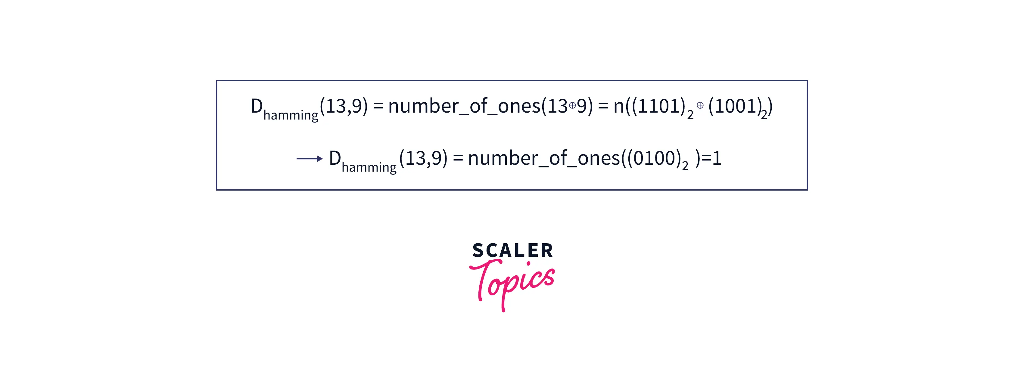
Hamming Distance is another distance metric computed by finding the bitwise XOR of 2 numbers and the number of 1s in the result. For example,
Euclidean distance is the most common distance metric, while the other metrics are used in niche problems. For example, the smallest path traveled by an airplane from point A to B on Earth is a curve since the Earth's curvature constrains the plane's movement.
Speeding Up KNN
KNN algorithm is non-parametric, which means there is no assumption for underlying data distribution. It is helpful in a real-world scenario where data do not follow theoretical assumptions. But, KNN is also a lazy algorithm, which means it does not need any training data points for model generation. All training data used in the testing phase. Hence, it makes training faster and the testing phase slower and costlier. Thus, to speed up KNN, several methods are proposed. We will discuss some of these methods in detail here.
KD Tree
In the KD Tree-based method, the training data is divided into multiple blocks. Next, instead of calculating distance with all the training data points, samples from the same blocks are considered.
How KD Tree Works:
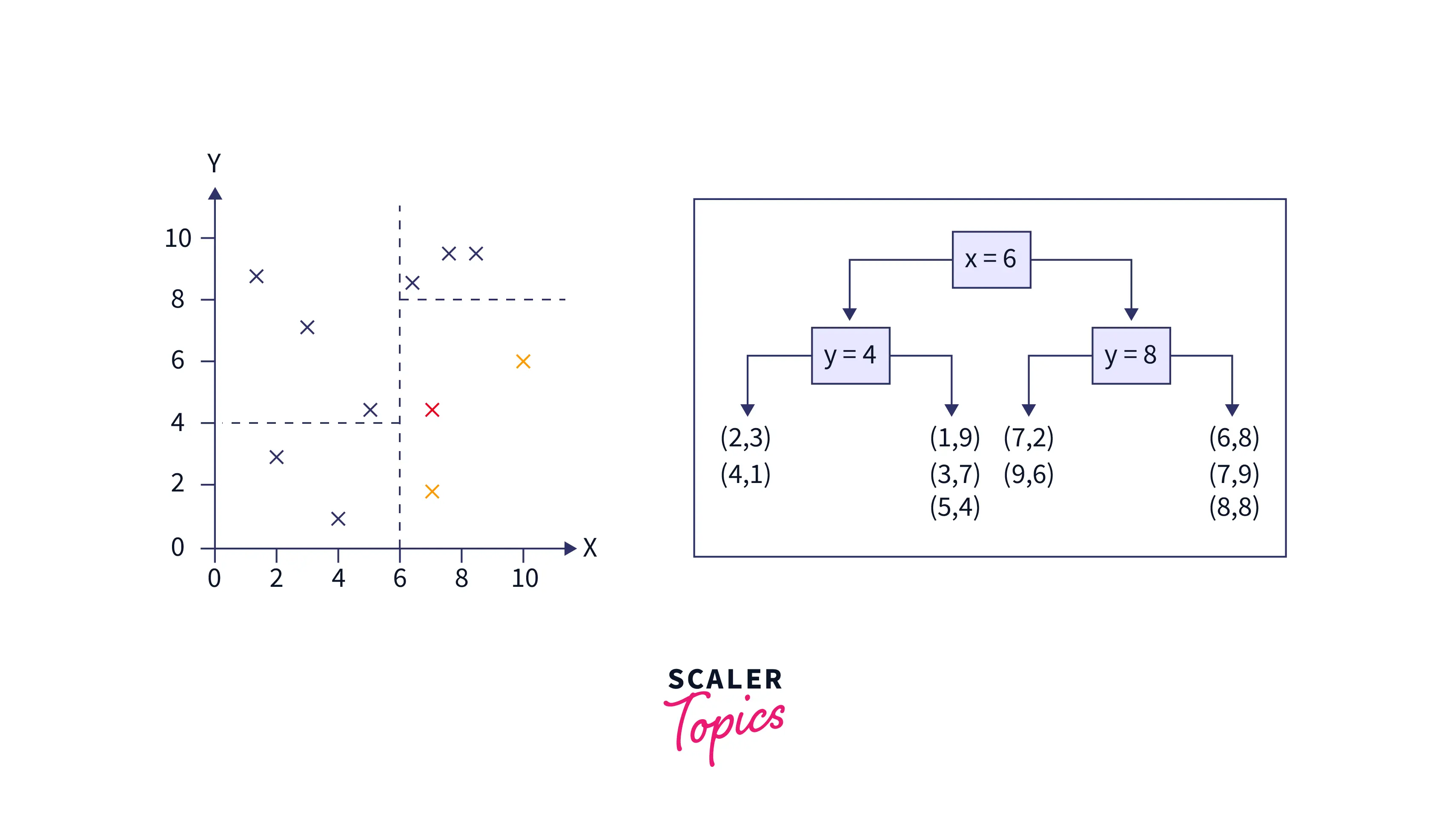
KD tree is built by splitting training data based on any random dimensions. For illustration purposes, let us try creating a KD tree for 2-dimensional data.
Consider training data as: (1,9), (2,3), (4,1), (3,7), (5,4), (6,8), (7,2), (8,8), (7,9), (9,6) - the steps to divide the data into several parts using KD Tree is shown below.
- Pick a split dimension :
Here, the x dimension is selected. X coordinate values for the data points are 1, 2, 4, 3, 5, 6, 7, 8, 7, and 9. - Find the median value:
Next, sorting the x coordinate data results 1, 2, 3, 4, 5, 6, 7, 7, 8, 9. The median value is 6. - Next, divide the data into approximately equal halves.
- Repeat steps 1 to 3: In the next iteration, the y coordinate is selected, its median is calculated, and data is again split. The second and third step is recounted to divide the data into multiple parts. The below graph shows that the space is first divided on x=6 and then on y=4, and y=8.
While testing, its distance is measured only with the samples of the same block to find the k nearest neighbors.
Turn Learning into Career Growth
Ball Tree
Ball Tree divides training data into circular balls (circular blocks). The similarity of the test data is calculated only with the training points in that block. Let's see how the ball tree is built.
First, the centroid of the entire training data is set. Then, the sample point farthest from the first centroid is selected as the center of the first cluster and child node. Next, the point furthest from the center of the first cluster is picked as the centroid of the second cluster. All other data points are assigned to cluster 1 or cluster 2. The method of dividing the data points into two clusters/spheres is repeated within each cluster until a depth. It creates a nested cluster containing more and more circles. Once clusters are built, they can intersect, but each point is assigned to one cluster. That is the concept behind the Ball Tree Algorithm.
Example:
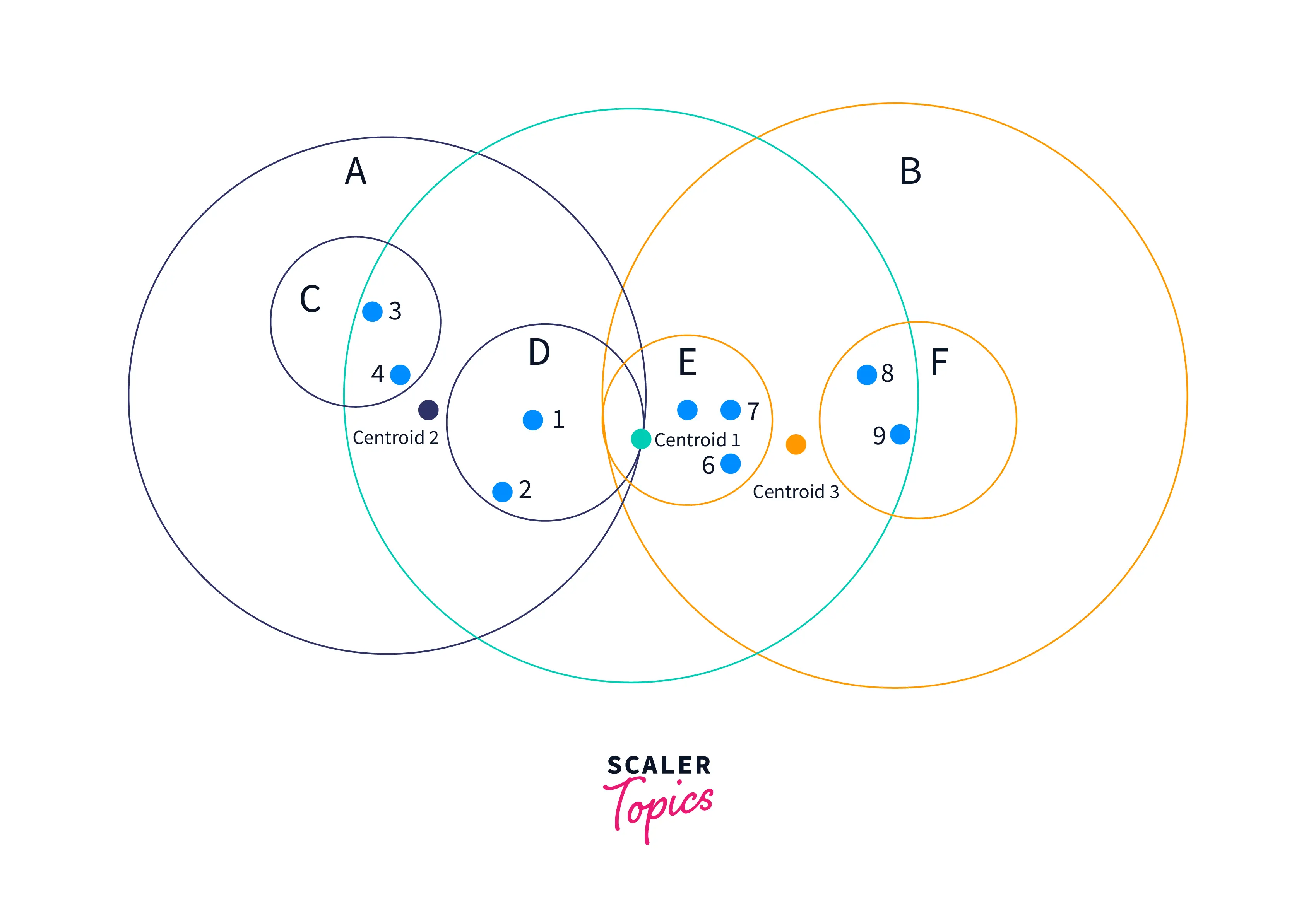
In the figure shown above, centroid 1 starts the algorithm. The gray sphere (2D) is laid around training data. From the center, the furthest point of a cluster is selected (number 3 or 9). The furthest point from number three is the center of cluster 2. The remaining clusters are constructed as discussed above.
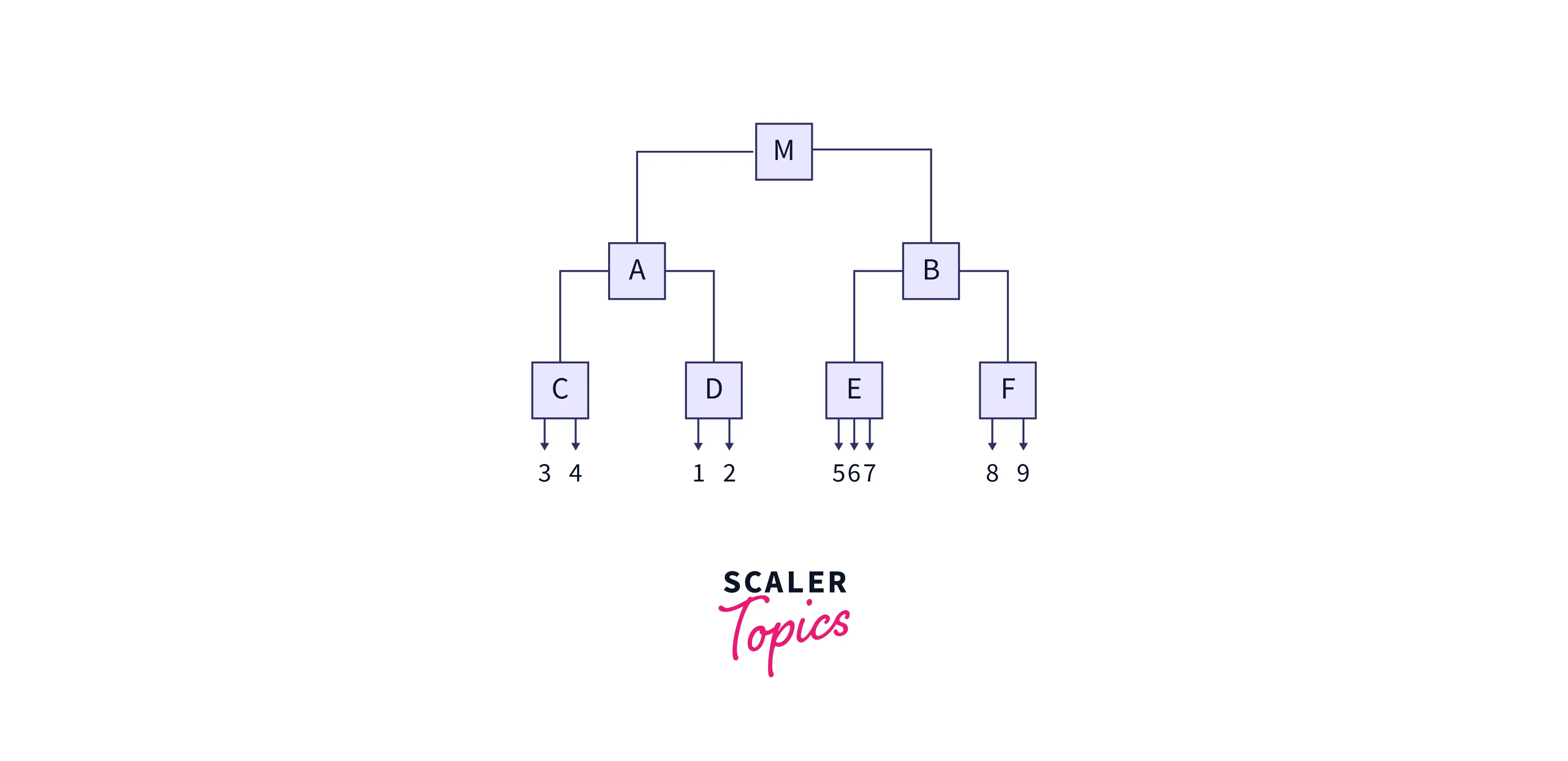
The resulting tree is shown below.
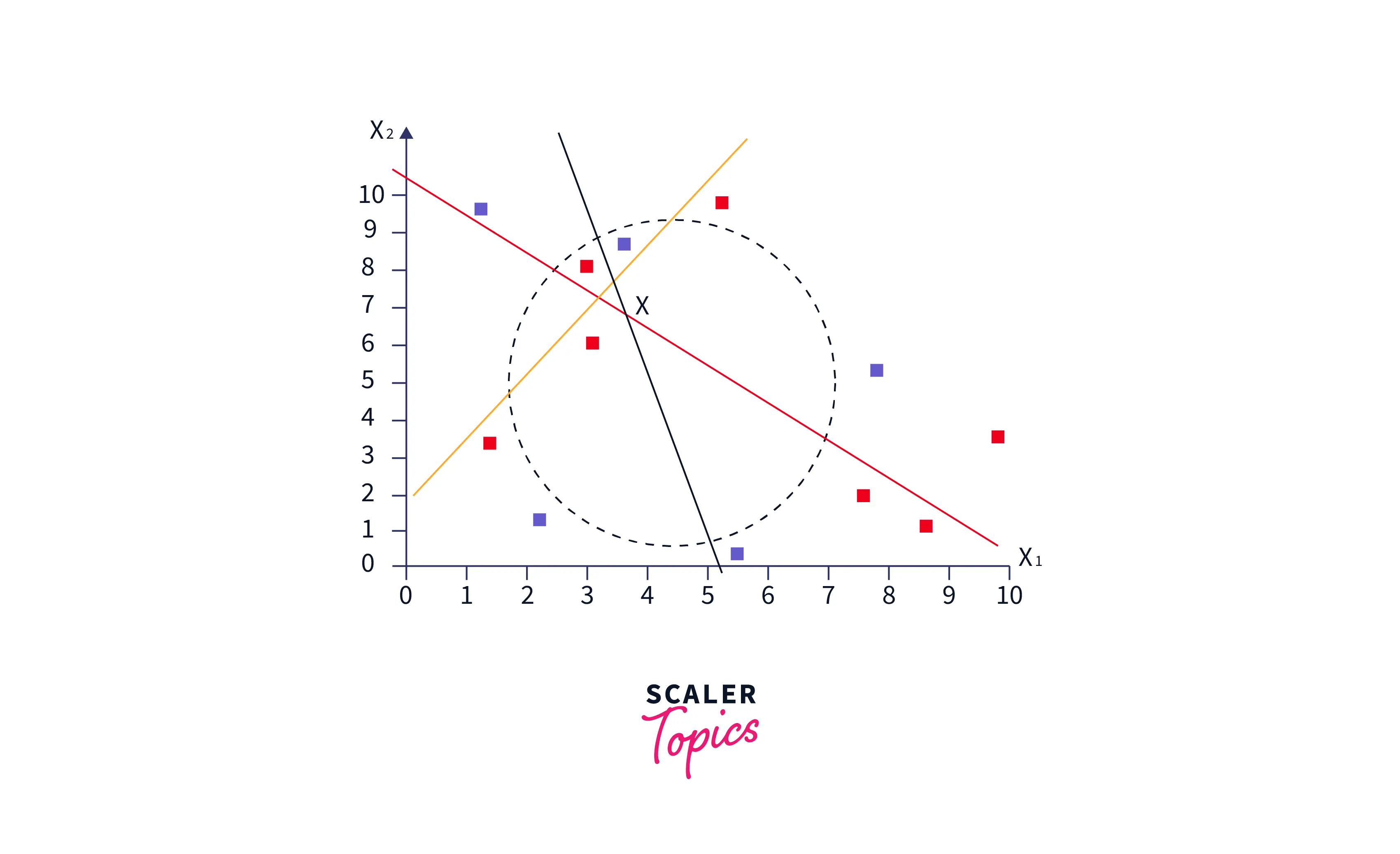
Approximate Nearest Neighbours
The approximate nearest neighbor algorithm provides another approach to speed up the inference time of the vanilla KNN algorithm with the help of the following steps.
- Randomly initialize a set of hyperplanes in the same space as the sample points. It will divide the plane into sub-spaces.
- Find out the subspace for each sample in training data.
- While inferencing, find the samples from the same subspace and treat them like neighbors.
- Next, calculate the distance between the test data and its new neighbors.
- Return the labels of the nearest K sample of the sub-space.
Curse of Dimensionality
It is observed that, for low dimensional data, some points remain close and few remain far from each other. However, all points are nearly equidistant in high dimensions, say d =100. The phenomenon is referred to as the Curse of Dimensionality.
It is a curse for KNN because, for large d, the idea of a k-nearest neighbor fails as the set of n points is nearly equidistant from one another. KNN needs all points to be close along every axis. Adding a new dimension makes it harder and harder for two specific points to be close to each other across every axis. Hence, the performance of KNN deteriorates with the increasing dimension.
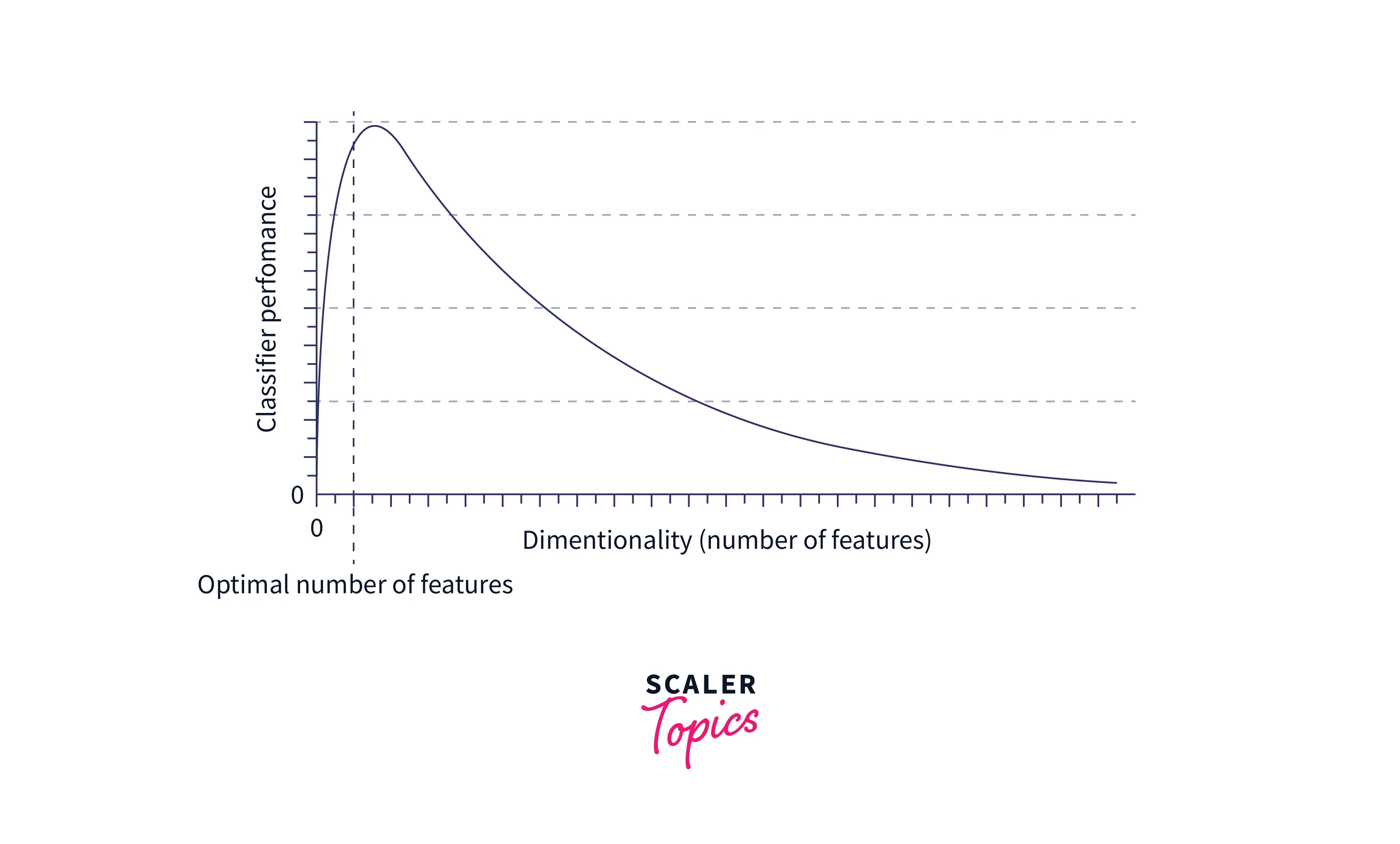
Solution
With the increasing dimension, KNN needs more data to maintain the density of points. Else it will lose all predictive power. Hence, adding more data is the most elementary solution to the problem of the curse of dimensionality for KNN. Unfortunately, however, adding more data is only sometimes possible because of either the unavailability of data or because it requires more memory to process the data. Hence, reducing the data dimension is another viable option to eliminate the problem.
Advantages of the KNN Algorithm in Machine Learning
- KNN is extremely useful in scenarios that require high accuracy and do not contain many unknown points to classify. The concept of learning does not apply to KNN. Hence, if we need a quick prediction for a limited number of data points, then KNN is the go-to algorithm since other models, like neural networks and logistic regression, require time for training.
- Easy to implement
- Simple hyperparameter tuning (unlike in neural networks)
Disadvantages of the KNN Algorithm in Machine Learning
- We can incorrectly classify something even if the confidence is 100% due to overfitting.
- KNN will confidently classify data points far beyond the dataset's actual scope.
- KNN is sensitive to noise, so accurate data preprocessing must be done.
- KNN employs instance-based learning and is a lazy algorithm that refers to an algorithm that does not learn anything from the dataset. Each time a new data point is supplied, it calculates the distance between that point and all other points in the dataset, which is computationally expensive. Essentially, the idea of training the KNN model does not exist because it makes a new decision by calculating the distances from a new point.
- For large datasets, the program needs to be memory-optimized, else it will take too much memory to perform classification. There are many workarounds for many of these disadvantages, which makes KNN a powerful classification tool. For example, we can apply the Weighted KNN algorithm to improve the accuracy. In addition, if the test dataset is large, we can use a mesh-grid that precomputes the predictions of data points and stores this result in a mesh.
Scaler Placement Report and Statistics
Scaler learners achieved 2.5x salary growth with average post-Scaler CTC reaching ₹23L.
Application of K-Nearest Neighbours
- KNN can be used in plagiarism checks to check if two documents are semantically identical.
- ML in healthcare uses KNN to diagnose diseases based on subtle symptoms.
- Netflix uses KNN in its recommendation systems.
- KNN is used in face recognition software.
- Political scientists and psychologists use KNN to classify people based on their behavior and response to stimuli.
Implementation of KNN Algorithm in Python
We’ll tackle the famous Iris Dataset to understand how KNN is implemented. It is highly recommended to implement KNN from scratch, as the algorithm is pretty simple. You can download the dataset from here.
First, read the data and generate train and test data using train_test_split of sklearn.
The output for the above code is shown below :
Next, let's try building a KNN model for K=5 and measure the accuracy of the model.
The code output is given below :
From this program, we get an accuracy of about 98% consistently for K = 5.
Unlock the power of mathematics in machine learning. Enroll in Maths for Machine Learning Course today!
Conclusion
- The k-Nearest Neighbors Algorithm is a fairly simple algorithm to understand and implement.
- While it is better to use libraries and well-developed tools, building it from scratch gives us a better perspective of how everything works under the hood and provides greater flexibility.
- Also, even though the KNN algorithm in machine learning has many shortcomings, it can be subsided with certain modifications and improvements, which makes it one of the most potent classification algorithms out there.