AVL Trees

What is AVL Tree
AVL (Adelson-Velsky and Landis) Tree is a self-balancing binary search tree that can perform certain operations in logarithmic time. It exhibits height-balancing property by associating each node of the tree with a balance factor and making sure that it stays between -1 and 1 by performing certain tree rotations.
This property prevents the Binary Search Trees from getting skewed, thereby achieving a minimal height tree that provides logarithmic time complexity for some major operations such as searching.
Balance Factor in Binary Search Tree
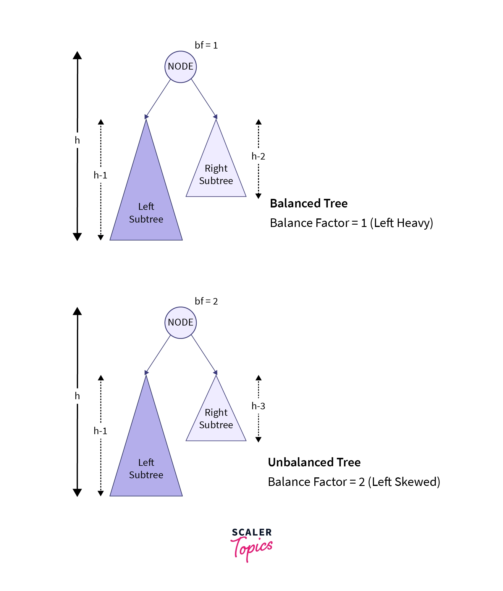
In an AVL tree, the balance factor of a node is the height difference between its left and right subtrees. It ensures the tree remains balanced, with a balance factor of 0 indicating equilibrium.
All nodes have balance factors within the range [-1, 1], indicating a balanced AVL tree. Mathematically, the balance factor (BF) of a node N is given by:
Transform Your Career
Choose from our industry-leading programs designed for career success
Modern Software and AI Engineering Program
Master full-stack development with AI integration

Modern Data Science and ML with specialisation in AI
Advanced data science techniques with AI specialization
Advanced AIML with Specialisation in Agentic AI
Deep dive into AIML with focus on Agentic systems
DevOps, Cloud & AI Platform Engineering
Build and manage AI-powered cloud infrastructure
AI Engineering Advanced Certification by IIT-Roorkee
Premier AI engineering certification from IIT-Roorkee
AVL Tree Rotation
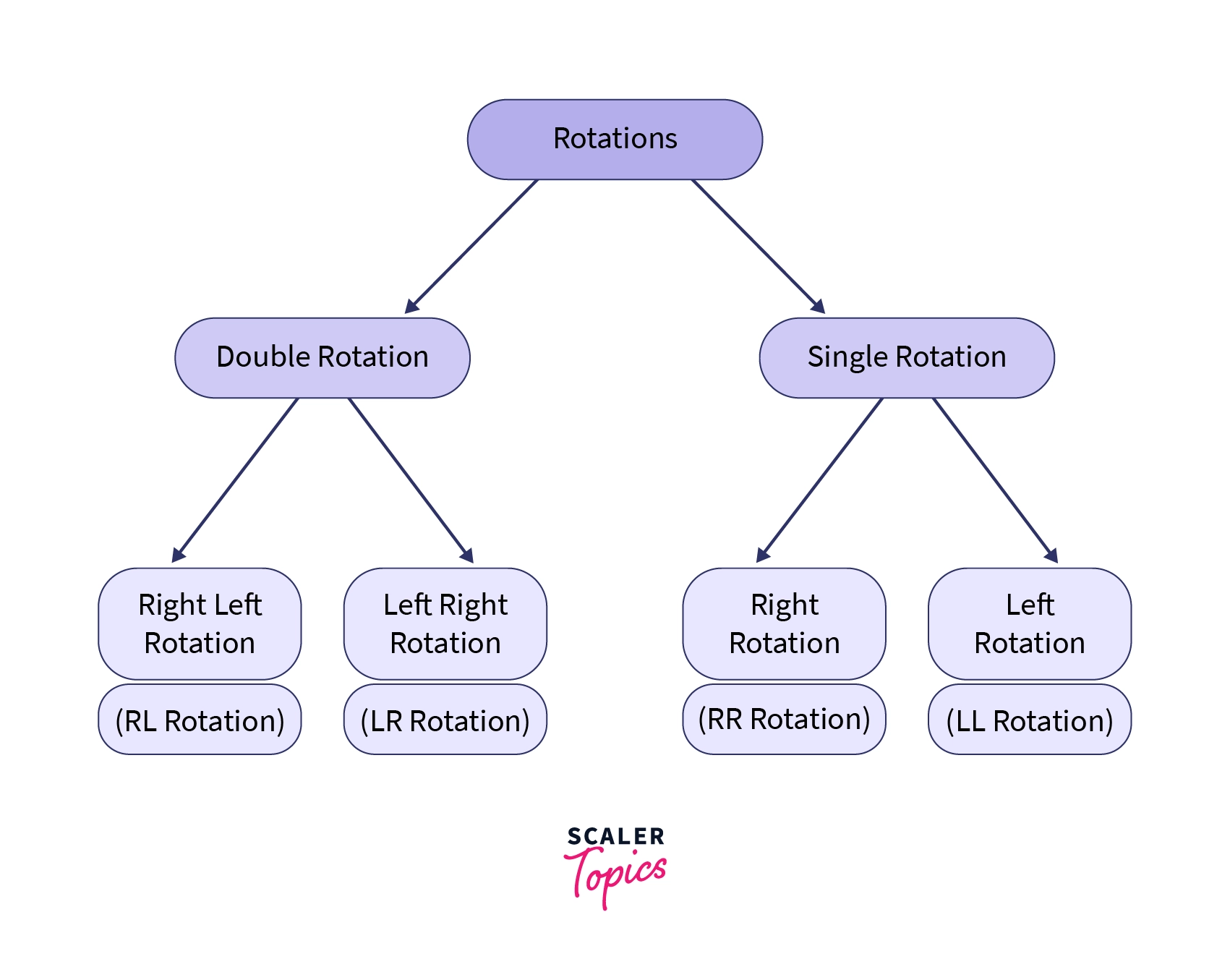
AVL Trees use a node’s balance factor to determine whether it is left-heavy, balanced, or right-heavy. When a node becomes unbalanced, an avl rotation is performed to restore balance. These rotations involve rearranging the tree structure without changing the order of elements. There are four types of rotations used, each targeting a specific node imbalance caused by changes in the balance factor.
These rotations include:
Now, let’s look at all the tree rotations and understand how they can be used to balance the tree and make it follow the AVL balance criterion.
1. LL Rotation
LL Rotation is a single rotation operation executed when the tree becomes unbalanced due to the insertion of a node into the left subtree of the left child of the node causing the imbalance, known as Left-Left (LL) insertion. This imbalance indicates that the tree is heavy on the left side. Hence, a single right rotation (or clockwise rotation) is applied such that this left heaviness imbalance is countered and the tree becomes a balanced tree. Let’s understand this process using an example:
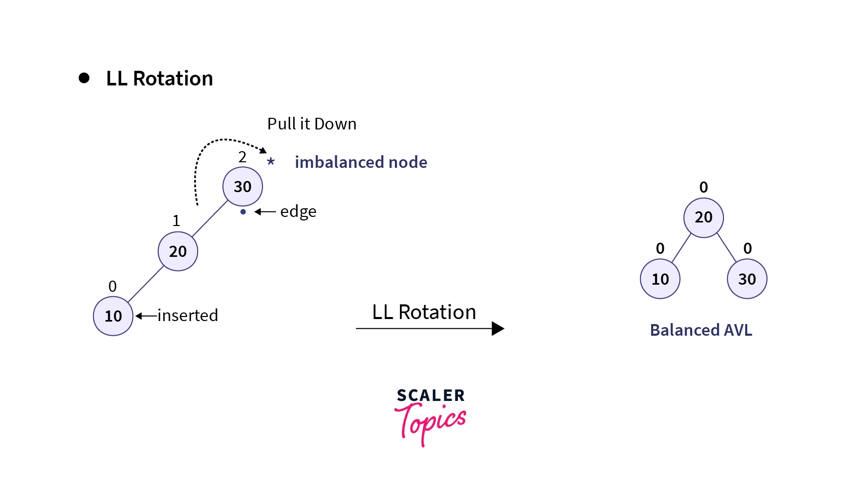
Calculating the balance factor of all nodes in the above tree, it is evident that the insertion of element 10 as the left child node along the left-child path has caused an imbalance in the root node, resulting in a left-skewed tree. This scenario represents a case of L-L insertion. To counteract the left skewness, a right rotation (clockwise rotation) is performed on the imbalanced node, where its left child node moves up and the original parent node shifts down to the right. This rotation shifts the heavier left subtree to the right side, restoring balance to the tree structure.
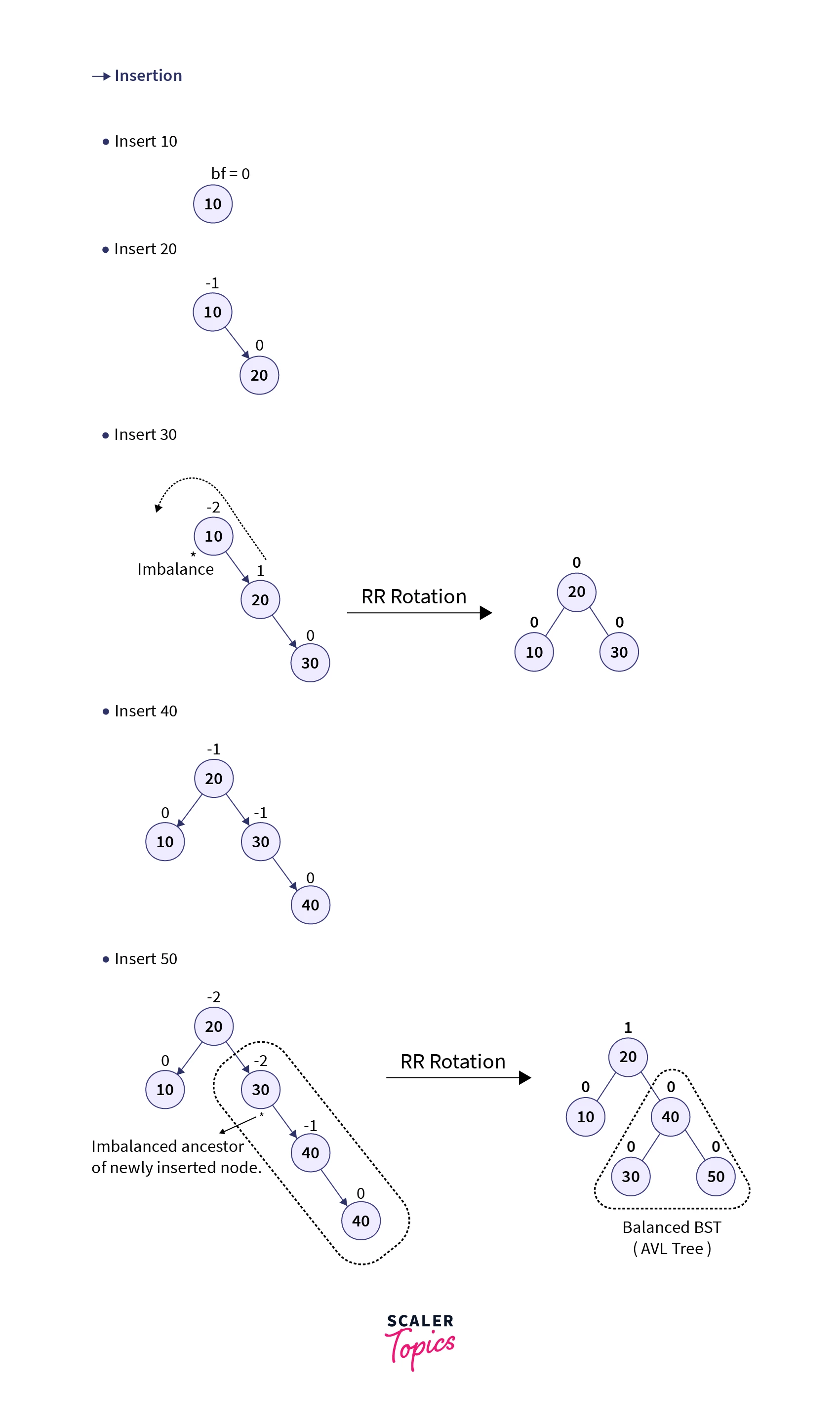
2. RR Rotation
It resembles the LL Rotation scenario, but here the imbalance arises when a node is inserted into the right subtree of the right child of the node causing the imbalance, and the standard single left rotation fix is used for Right-Right (RR) insertion, contrasting with the LL insertion. In this case, the tree becomes right heavy because the new key is added as the right child node along the right child path, and we left rotate the imbalanced node to counter this right skewness caused by the insertion operation. Let’s understand this process with an example:
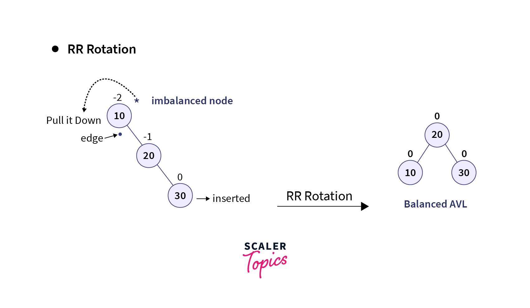
Upon calculating the balance factor of all the nodes, we can confirm that the root node of the tree is imbalanced (balance factor = 2) when the element 30 is inserted using RR-insertion.
3. LR Rotation
The left right case arises when a node is inserted into the right subtree of the left child of a node that is already imbalanced. This situation can be illustrated with the example of creating a BST using elements 30, 10, and 20. Upon insertion of element 20 as the right child of the node with value 10, the tree becomes imbalanced with the root node having a balance factor of 2.
Positive balance factors indicate left-heavy nodes, while negative balance factors indicate right-heavy nodes.
Now, if we notice the immediate parent of the inserted node, we notice that its balance factor is negative i.e., its right-heavy. Hence, the first correction is a left right rotation sequence, beginning with a left rotation on the left child of the unbalanced node. Let’s perform this rotation and notice the change:
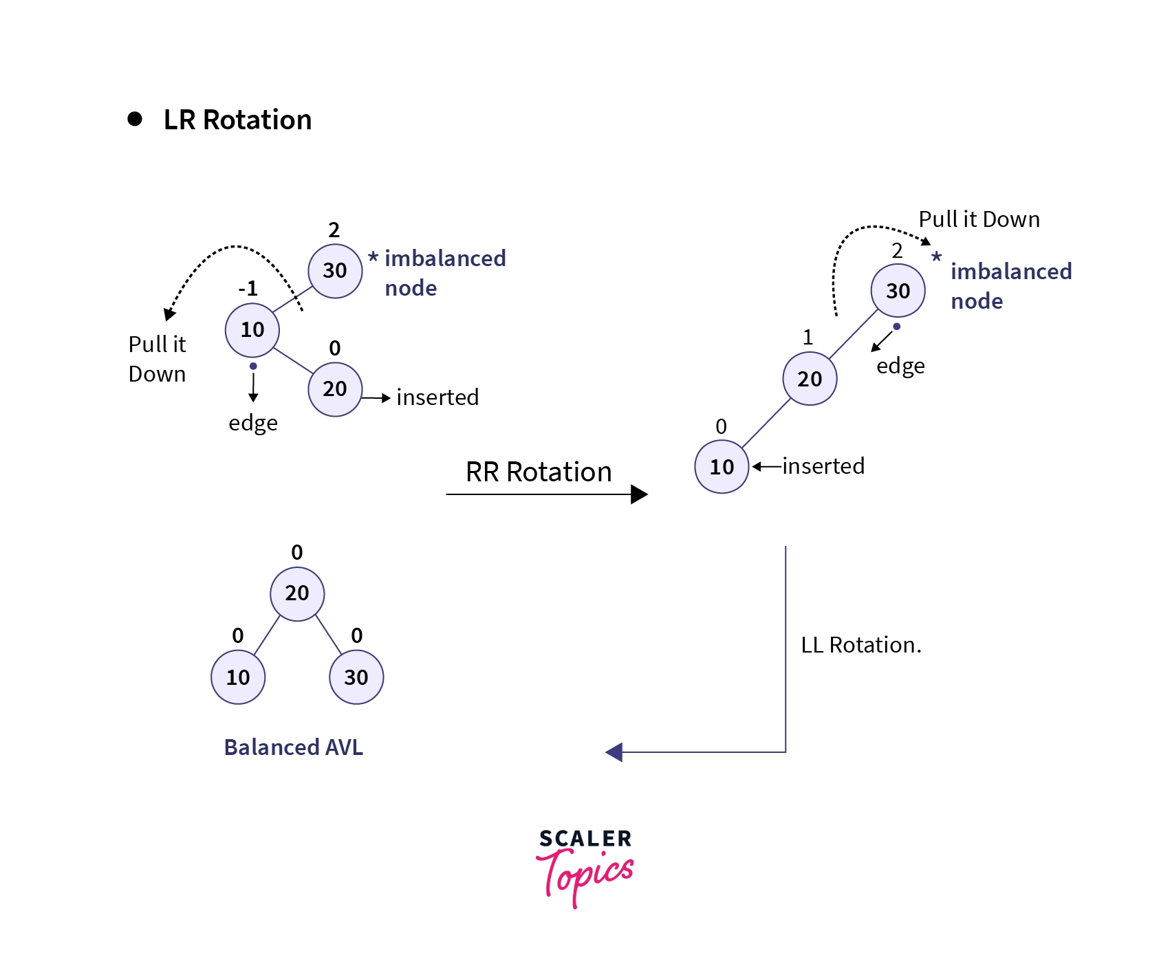
As you can observe, upon applying the RR rotation the BST becomes left-skewed and is still unbalanced. This is now the case of LL rotation and by rotating the tree along the edge of the imbalanced node in the clockwise direction, we can retrieve a balanced BST.
This process of applying two rotations sequentially one after another is known as double rotation and, for the LR order, we first rotate left on the left child and then rotate right on the unbalanced node to restore balance.


4. RL Rotation
It is similar to LR rotation but it is performed when the tree gets unbalanced upon insertion of a node into the left subtree of the right child of the imbalance node, i.e., upon Right-Left (RL) insertion instead of LR insertion. This case is corrected with a right left rotation: first, a right rotation is performed on the right child of the unbalanced node, followed by a left rotation on the unbalanced node to restore balance.
Let’s now observe an example of the RL rotation:
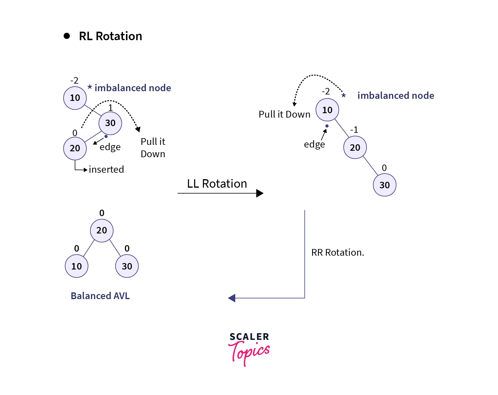
In the above example, we can observe that the root node of the tree becomes imbalanced upon insertion of the node having the value 20. Since this is a type of RL insertion, we first perform a right rotation on the immediate parent of the inserted node and then a left rotation around the imbalanced node (in this case the root node) to get the balanced AVL tree.
Operations on AVL Trees
Since AVL Trees are a self balancing bst and a balancing bst, all the operations carried out using AVL Trees are similar to those of Binary Search Trees. Also, since searching an element and traversing the tree don’t lead to any change in the structure of the tree, these operations can’t violate the height balancing property of AVL Trees, and faster lookups follow because the tree height stays smaller. Hence, searching and traversing operations are the same as those of Binary Search Trees. In avl tree compared with a regular BST, the only difference is the rebalancing rotations that prevent degeneration into a linear linked-list-like unbalanced tree.
Scaler Placement Report and Statistics
Scaler learners achieved 2.5x salary growth with average post-Scaler CTC reaching ₹23L.
1. Insertion
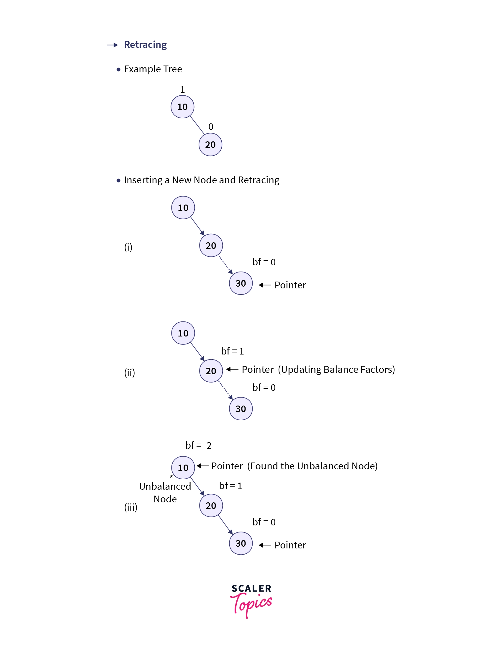
In Binary Search Trees (BSTs), a new node (let’s say N) is inserted as a leaf node by replacing the NULL value of a node’s child. Similarly, in AVL Trees, the new node is also inserted as a leaf node, with its balance factor initially set to 0. However, after each insertion, the balance factors of the ancestor nodes of the newly inserted node are checked to ensure tree balance. Only the ancestors are examined because the insertion only affects their heights, potentially inducing an imbalance. This process of traversing the ancestors to find the unbalanced node is called retracing. During avl tree insertion, heights are updated and the avl invariant is checked on each ancestor node until balance is restored.
If the tree becomes unbalanced after inserting a new node, retracing helps us in finding the location of a node in the tree at which we need to perform the tree rotations to balance the tree.
Let’s look at the algorithm of the avl tree insertion operation in AVL Trees:
Insertion in AVL Trees:
-
START
-
Insert the node using BST insertion logic.
-
Calculate and check the balance factor of each node.
-
If the balance factor follows the AVL criterion, go to step 6
-
Else, perform tree rotations according to the insertion done. Once the tree is balanced go to step 6.
-
END
For better understanding let’s consider an example where we wish to create an AVL Tree by inserting the elements: 10, 20, 30, 40, and 50. The below gif demonstrates how the given elements are inserted one by one in the AVL Tree, ending with the balanced final tree after rebalancing:
2. Deletion
When an element is to be deleted from a Binary Search Tree, the tree is searched using various comparisons via the BST rule till the currently traversed node has the same value as that of the specified element. If the element is found in the tree, there are three different cases in which the delete operations occur depending upon whether the node to be deleted has any children or not:
Case 1: When the node which has to be deleted is a leaf node
- In this case, the node to be deleted contains no subtrees i.e., it’s a leaf node. Hence, it can be directly removed from the tree.
Case 2: When the node to be deleted has one subtree
- In this case, the node to be deleted is replaced by its only child thereby removing the specified node from the BST.
Case 3: When the node to be deleted has two children.
-
In this case, the node to be deleted has two child nodes and can be replaced by one of the two available nodes:- It can be replaced by the node having the largest value in the left subtree (Longest left node or Predecessor).
-
Or, it can be replaced by the node having the smallest value in the right subtree (Smallest right node or Successor), which also matches the in order traversal view of BST ordering.
Let’s look at the algorithm of the deletion operation in AVL Trees:
Deletion in AVL Trees
-
START
-
Find the node in the tree. If the element is not found, go to step 7.
-
Delete the node using BST deletion logic.
-
Calculate and check the balance factor of each node.
-
If the balance factor follows the AVL criterion, go to step 7
-
Else, perform tree rotations to balance the unbalanced nodes. Once the tree is balanced go to step 7
-
END
Like insertion, delete operations may require rebalancing up the tree.
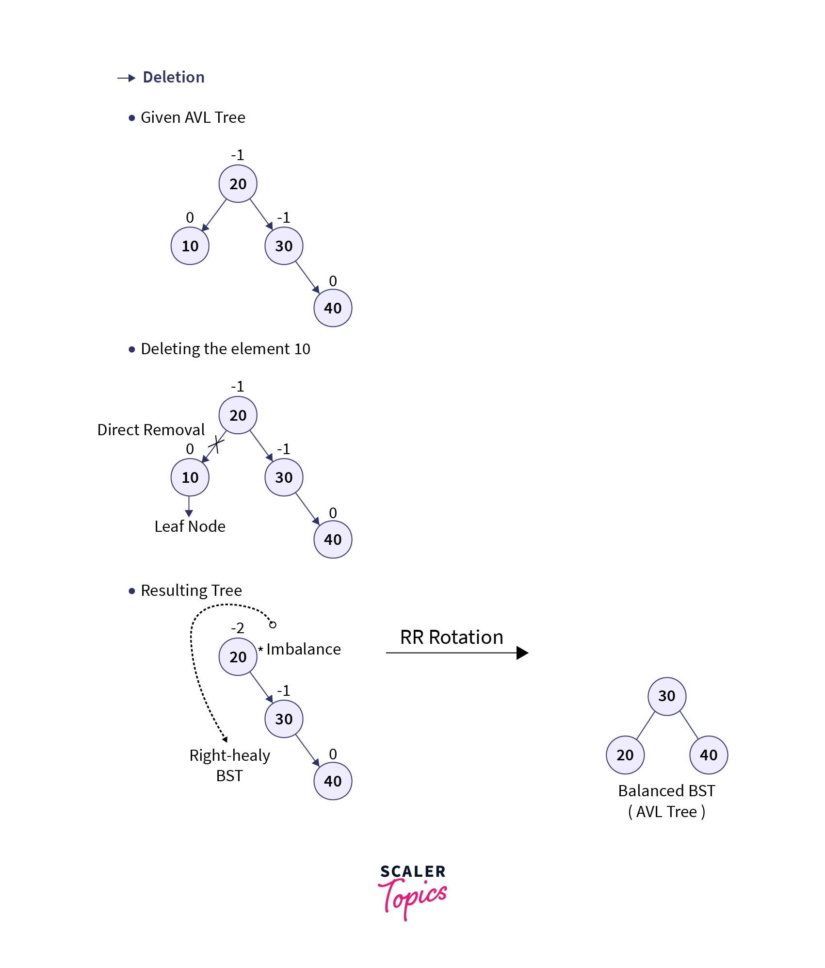
For better understanding let’s consider an example where we wish to delete the element having value 10 from the AVL Tree created using the elements 10, 20, 30, and 40. The below gif demonstrates how we can delete an element from an AVL Tree:
Code Implementation
Java
Here is an avl tree implementation in Java that covers insertion, height updates, and balancing rotations.
Turn Learning into Career Growth
C++
Python
Output:
Complexity Analysis
Time Complexity:
-
Insertion, Deletion, Search:
-
Average Case: O(log n)
-
Worst Case: O(log n)
-
Explanation: AVL tree operations maintain a balanced structure, ensuring logarithmic time complexity for insertion, deletion, and search operations. Rebalancing steps, if required, contribute only O(1) time per level.
-
Space Complexity:
-
Average Case: O(n)
-
Worst Case: O(n)
-
Explanation: AVL trees require space proportional to the number of nodes 'n'. Each node stores data and references to its children, resulting in O(n) space complexity. Additionally, recursive function calls during tree operations consume stack space, but it remains within O(n).
Applications of AVL Tree
-
Indexing large records in databases for efficient searching.
-
Handling in-memory collections like sets and dictionaries.
-
Database applications requiring frequent data lookups over insertions and deletions.
-
Software requiring optimized search capabilities.
-
Corporate environments and storyline games leverage AVL trees for their efficiency in managing and retrieving data.
Advantages of AVL Tree
-
Self-balancing property ensures optimal tree structure.
-
Absence of skewness guarantees balanced branching.
-
Faster lookup operations compared to Red-Black Trees.
-
Improved searching time complexity compared to binary trees.
-
Height remains bounded by log(N), enhancing overall efficiency.
Disadvantages of AVL Tree
-
Complex implementation process.
-
High constant factors for certain operations.
-
Less popular compared to Red-Black trees.
-
Complicated insertion and removal due to strict balance requirements.
-
Increased processing overhead for balancing operations.
-
AVL Trees are self-balancing binary search trees designed to maintain logarithmic time complexity for insertion, deletion, and search operations.
-
They utilize balance factors to ensure each node's height difference between left and right subtrees stays within a balanced range.
-
AVL Trees employ rotations, including LL, RR, LR, and RL rotations, to restore balance when nodes become unbalanced due to insertions or deletions.
-
These rotations involve rearranging the tree structure without changing the order of elements, ensuring efficient balancing while preserving the tree's properties.
-
Despite their efficient performance, AVL Trees require careful implementation and incur higher constant factors for certain operations.
-
While not as widely used as Red-Black Trees, AVL Trees find applications in databases, in-memory collections, and software requiring optimized search capabilities.