Biconnected Components

Biconnected Graph

A graph is a Biconnected graph if:

• There is a path from any node to any other node, i.e. the graph must be connected.
• After removing any node and all the associated edges from the graph, it still remains connected, i.e. there is always a path between any two nodes even after removing any node from the graph.
• For example consider the graphs below,

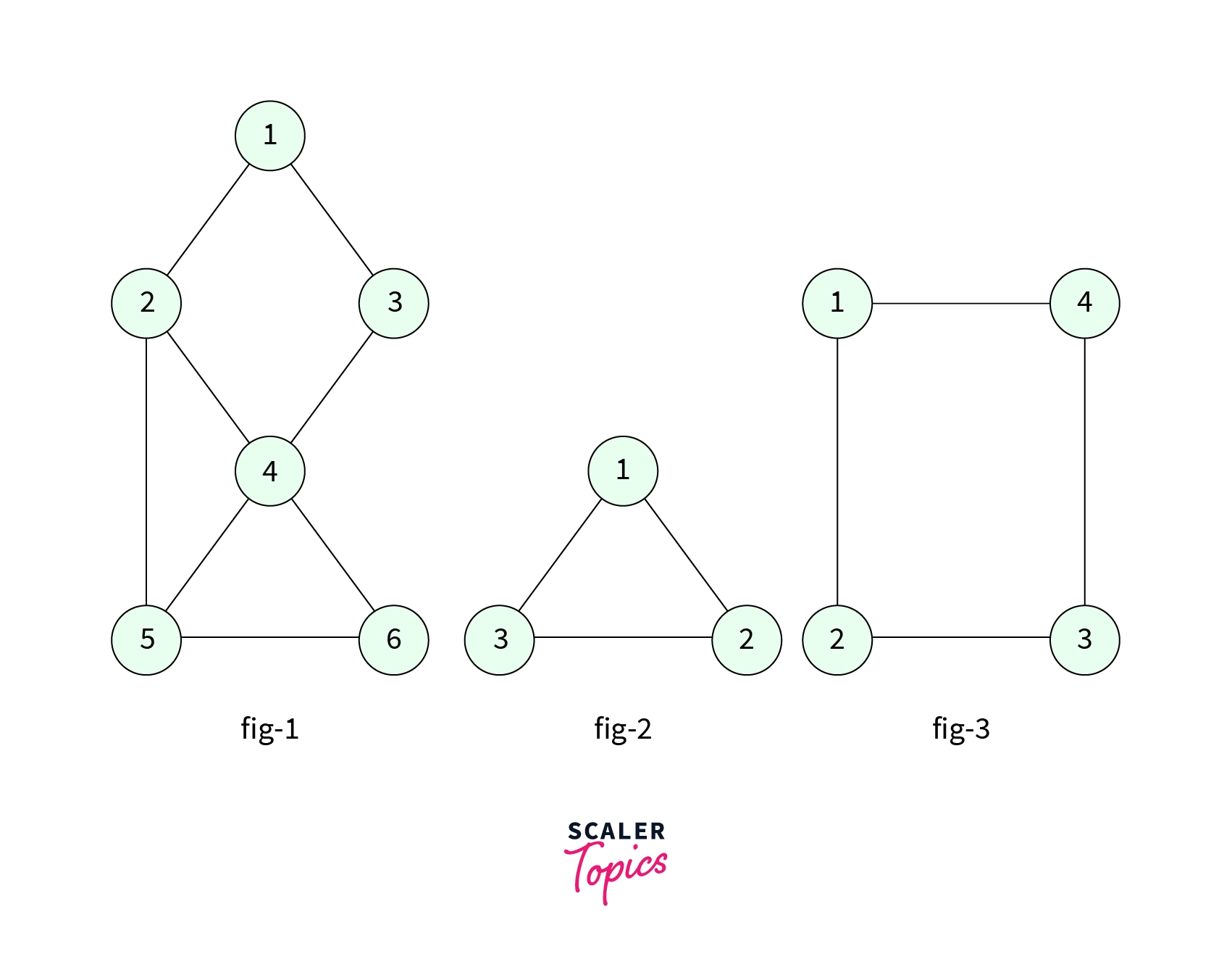
You can try and remove every possible node from any graph, it always remains connected. And also all of the graphs are one single component, there is a path from any node to any other node.

• Consider the graph shown below, it is not a Biconnected graph because if we remove the node with value 2, it increases the number of connected components and there is no edge between node 1 and node 5, or node 4 and node 6 etc.

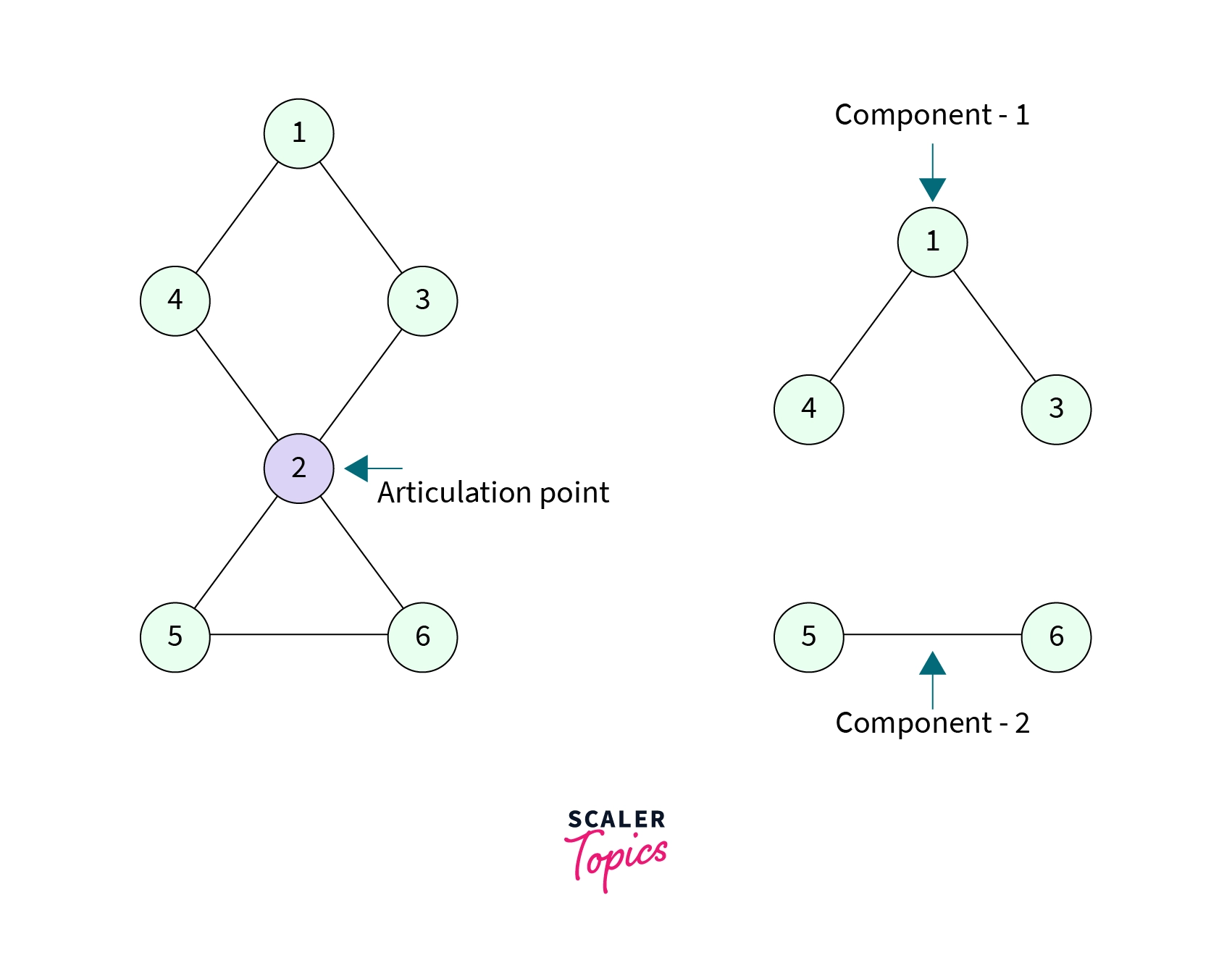
• A node whose removal from the graph increases the number of connected components is called an Articulation Point. In the above graph, the node with value 2 is an articulation point.
• A graph can contain multiple articulation points. We will also discuss the algorithm to detect the articulation points in a graph.
• To check whether a graph is Biconnected or not, we mainly need to check two things in a graph,
  • The graph is connected, i.e. there must be a path between any two nodes in the graph.
  • There is no articulation point in graph, as discussed above that a Biconnected graph has no articulation points.

Algorithm to Detect Articulation Point in a Graph

The algorithm to detect the articulation point in a graph is purely based on depth-first-search(DFS) which is a common traversal algorithm in graph data structure. Let's discuss some terminologies that we will be using to detect the articulation point,

1. Discovery Time(disc[node]): It is the time when a particular node is visited in a DFS call. It always starts with 1 (for the sake of implementation, since all we care about is which node is discovered when) and is incremented by 1 as we visit a new node in the DFS call.
   • To record the discovery time of each node in the graph we will be using an array disc[] of size equal to the number of nodes in the graph.
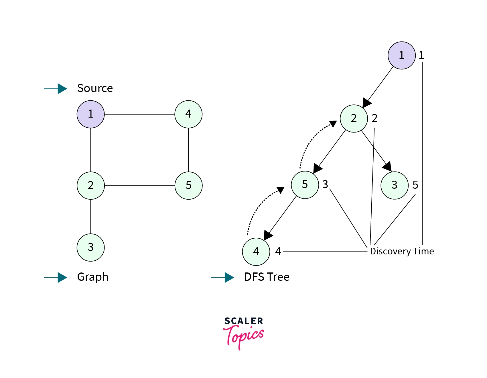
   • In the graph below, we assign discovery time to each node if a DFS call is made to source node 1. The DFS tree explains the order in which the nodes are visited in DFS call.

2. Parent Array(par[node]): We will also maintain a parent array to keep track of the parent of each node. Parent[i] for a node i determines from which node did the DFS call has been made to node i. Source node has parent = -1.
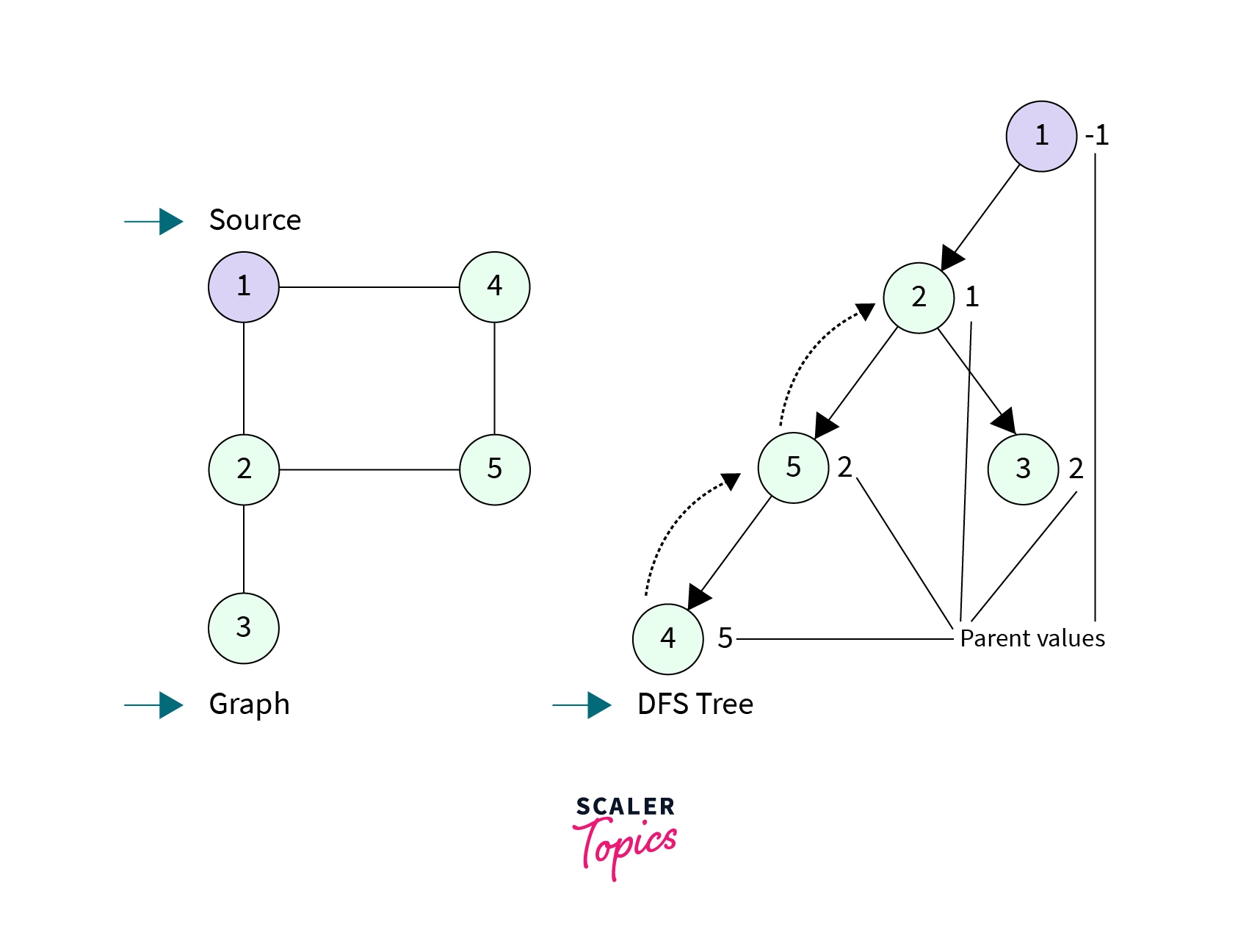
   • In the below graph value written to the side of the node are the parent values of that node.
   • Node 2 has a parent value equal to 1, which is indeed the node that made the DFS call to node 2. Node 2 then made DFS call to node 5 and node 3, that's why their parent values are 2.

3. Lowest Reachable Ancestor(low[node]): The low value of a node is the lowest possible discovery time of a previously discovered node if we ignore the current DFS path.

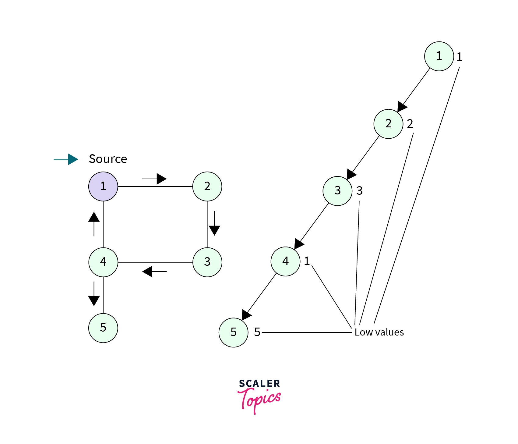
• Consider the above graph, if the source node is 1 then
  • Low[1] = 1, because it is the first node to be discovered in DFS call
  • Low[2] = 2, because there is no other path leading to any other previously discovered node except the current path.
  • Low[3] = 3, because there is no other path leading to any other previously discovered node except the current path.
  • Low[4] = 1, because there is a path from node 4 to node 1, which is not the current DFS path and is leading to a previously discovered node.
  • Low[5] = 5, because there is no other path leading to any other previously discovered node except the current path.

Algorithm to find the Articulation Point

1. Take a source node and make a DFS call, assign both the low[] value and disc[] time equal to time, as disc[] will not change but low[] value might change when we backtrack from a node in DFS call. In graph there are multiple paths to visit the same node and it might affect the discovery time of the node, so to make sure that we always keep the lowest low[] time for each node we update the low[] value while returning from DFS call.
2. When we visit a neighbor in the DFS call one of the three conditions will be true,
   • If the neighbor is the parent node, then
     • Continue to next neighbor, because we don't want to visit the node again which is already visited and the parent is already visited.
   • If the neighbor is not a parent but already visited
     • Reassign the low value of the current node with the minimum of low[] value of the current node and disc[] value of neighbor.
     • low[current_node] = minimim_of(low[current_node], disc[neighbour])
     • The reason why we did this is that there might be a possibility to get a less low[i] time for a current node i and low[i] is the lowest possible discovery time of node i.
   • Neighbour is not visited, of course, not a parent as well
     • Make DFS call to the neighbor
       • DFS(neighbour)
     • While returning from DFS call, update low[] value
       • low[current_node] = minimim_of(low[current_node], low[neighbour]), same as we discussed in the first step.
     • Now it's time to detect the articulation point
       • If the current node is the parent node, (par[current_node] = -1), then count the number of DFS calls made from the parent. If the count is greater than 1, then the current node is an Articulation point.
       • Because if it's a parent node and count of DFS calls is greater than 1, then more than 1 DFS call is being made from the source node, which is only possible when source node is the only junction between two components of a graph.
       • If the current node is not the parent node, then check if (low[neighbout] >= disc[current_node]) if this is true then, current node is an Articulation point.

Time Complexity of detecting Articulation Points: If you closely observe we are only visiting each node once and in depth-first-search manner. So the time complexity to detect the articulation points in a graph is O(V + E), which is the same as the time complexity of DFS traversal in a graph. V is the number of nodes and E is the number of edges in the graph.

Below is a DFS tree for the graph along with the discovery time and low value for each node.

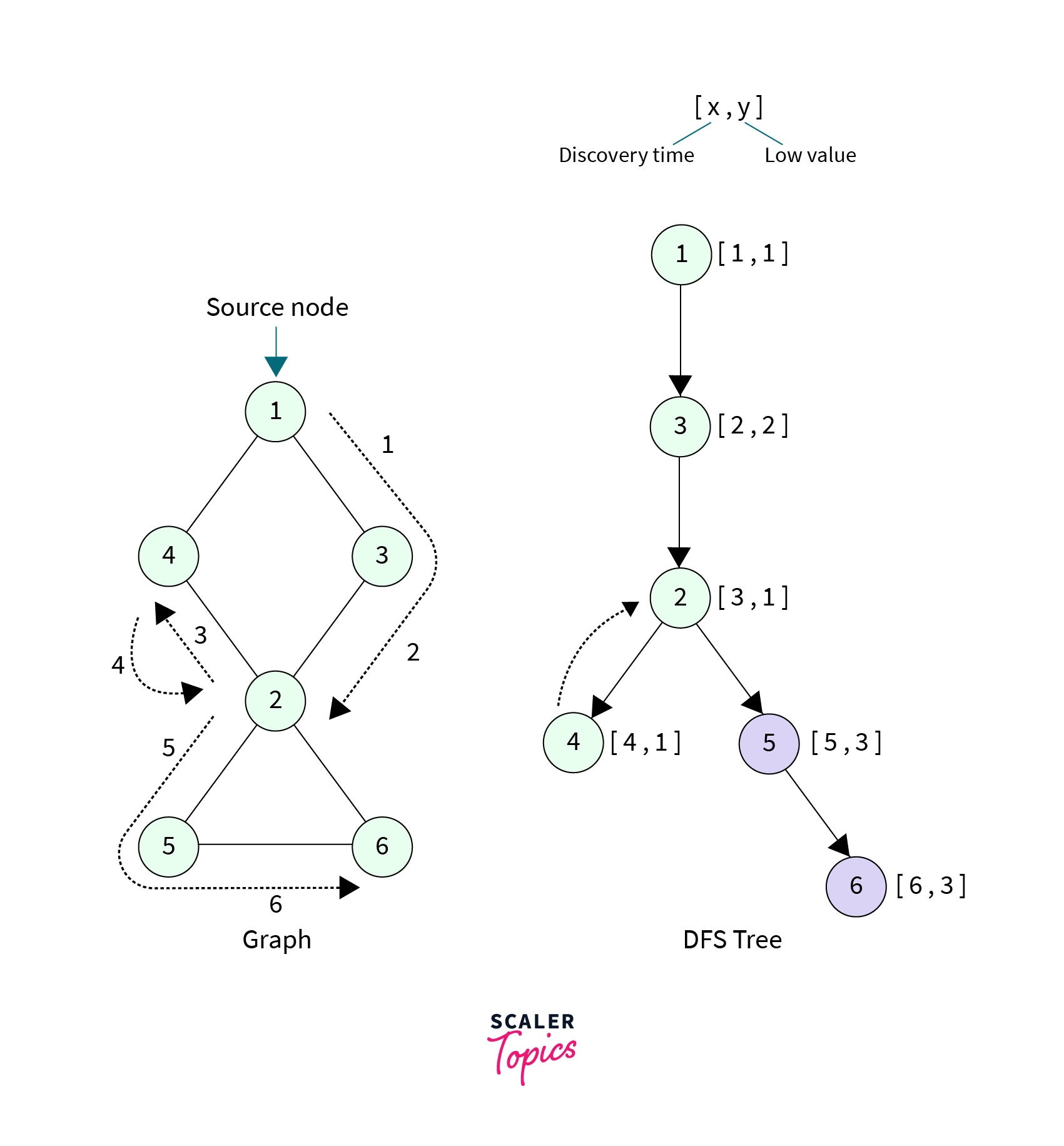
Clearly node 2 and it's neighbour 5, low[5] >= disc[2], so that mean node 2 is an Articulation point and our algorithm returns true.

Now let's head back to Biconnected components, I promise things will be much easier now.

Biconnected Components

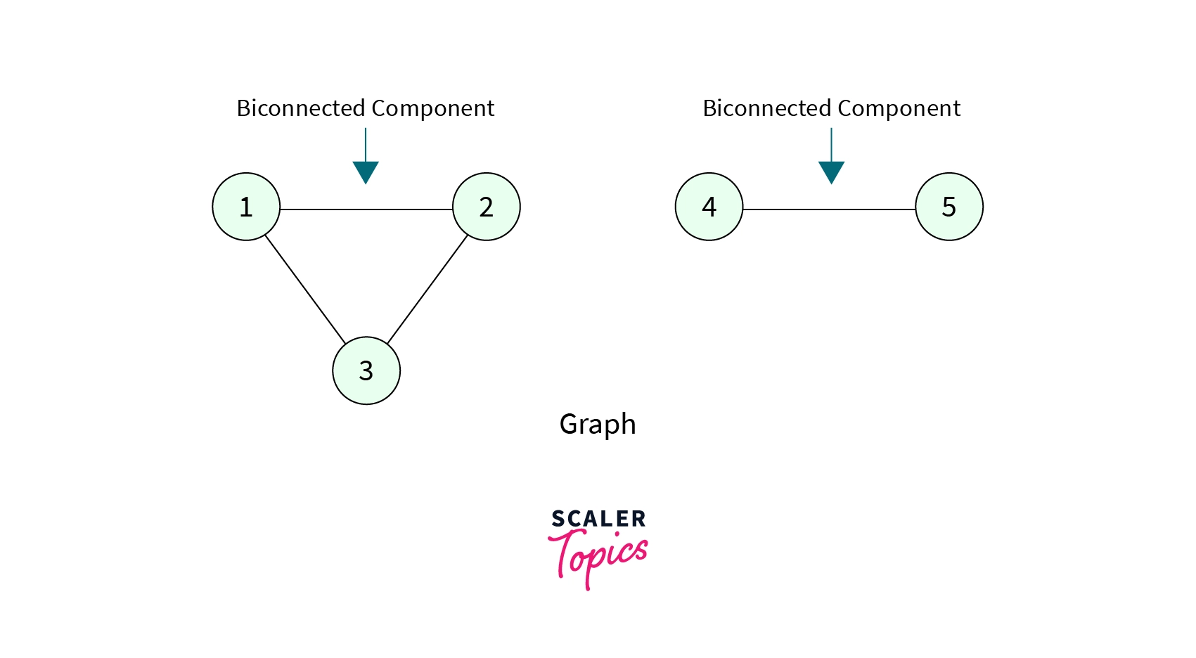
• For a given graph, a Biconnected Component is one of its subgraphs that is Biconnected. This means there is always a path between any two nodes in the component, even after removing any node from the component.

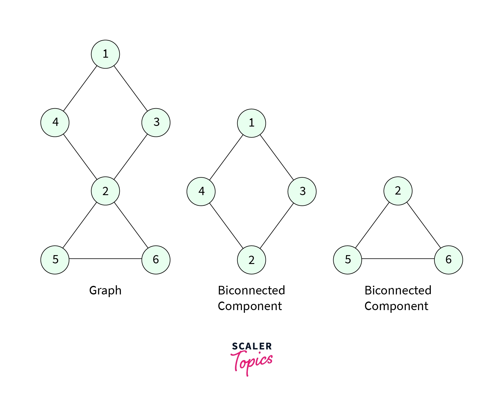
For example, for the graph given, it has 2 bioconnected components.

• Biconnected components in a graph can be easily determined with the help of the same algorithm we used to detect the Articulation point. Remember we return true as soon as we detect an Articulation point, let's take advantage of this fact.
• We maintain a stack of edges. Why only stack? because we want quick insertion and deletion operations and stack provides both insertion and deletion in constant time. Each element in the stack will refer to an edge U -> V, where U is the source and V is the destination.
• Keep adding edges to the stack in the order they are visited and when an articulation point is detected i.e. say a node U has a childV such that no node in the subtree rooted at V has a back edge (low[V] >= disc[U]) then pop and print all the edges in the stack till the edge U-V is found, as all those edges including the edge U-V will form one biconnected component.

Example of Biconnected Components Algorithm

• Consider the graph shown below, let's do a dry run of the algorithm we discussed above.

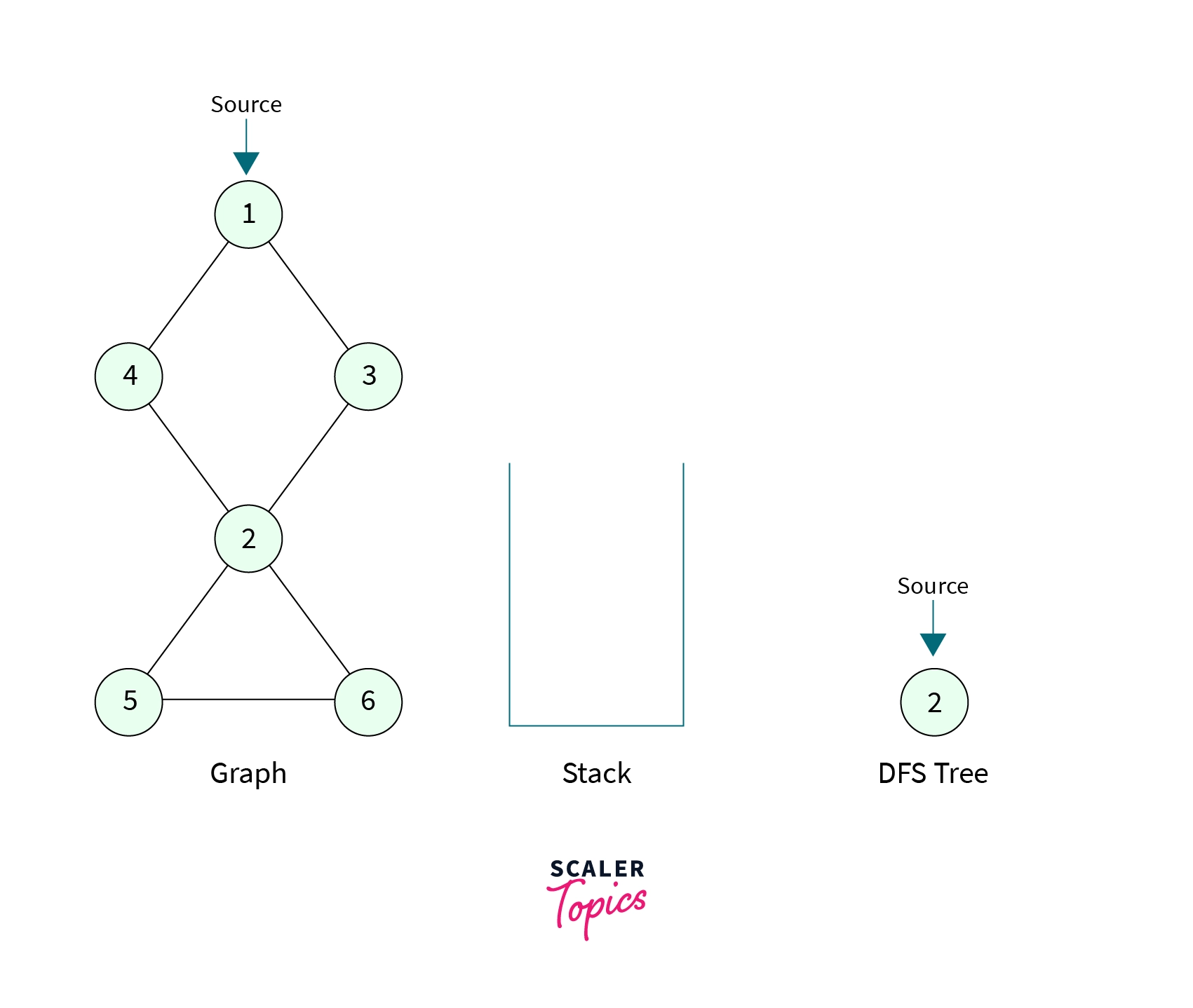
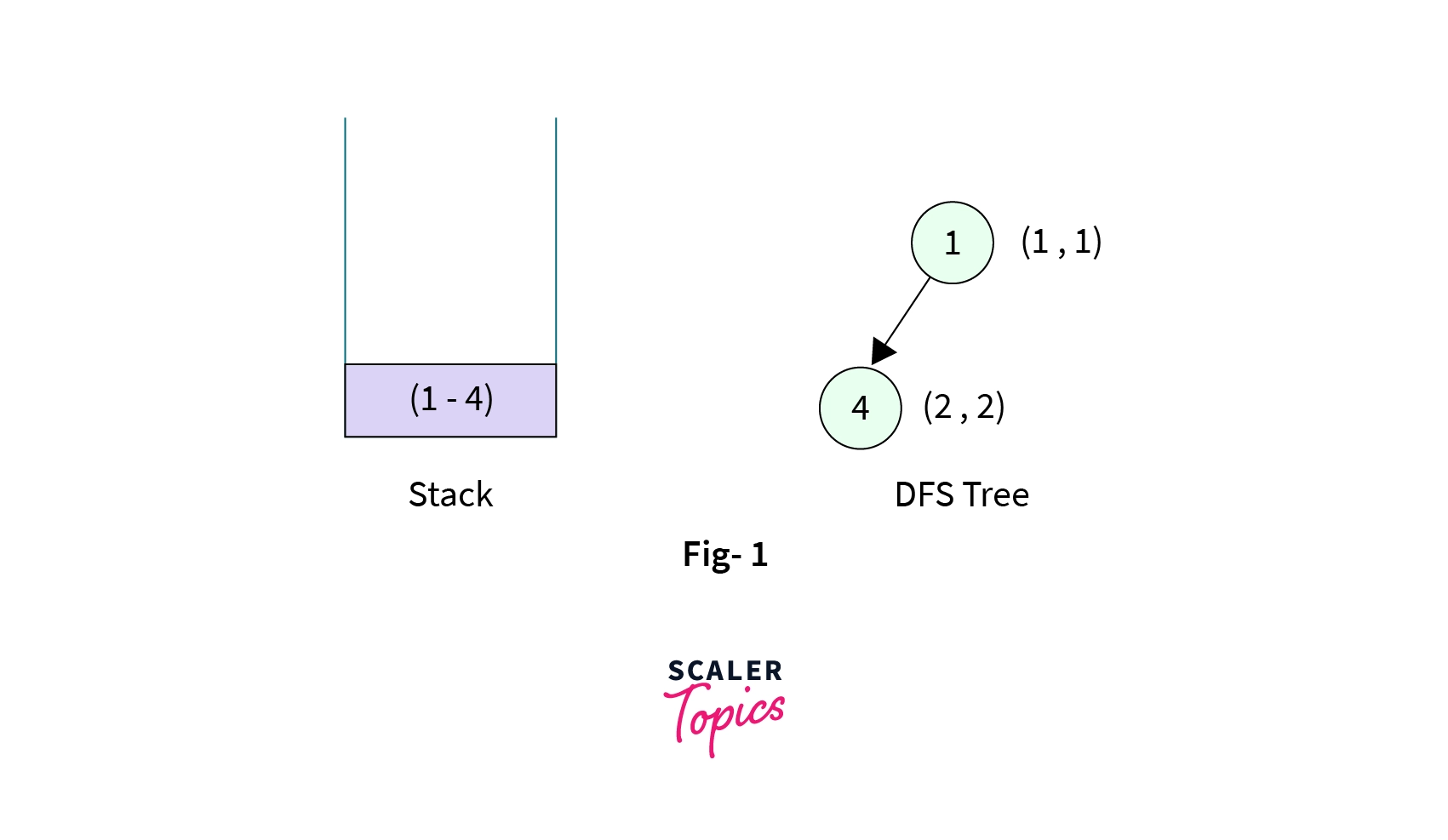
• Suppose the source node is the node with the value 1. First, we make a DFS call to this node with an empty stack. We mark Node-1 as visited, discovery time, and low time as (1, 1) and now we have to make a DFS call to one of its unvisited children. Node-1 has two children(Node-4 and Node-3), suppose DFS call is then made to Node 4. Node 4 is marked visited with discovery time and low time as (2, 2) and the edge from Node-1 to Node-4 is pushed into the stack. The stack now contains one element,

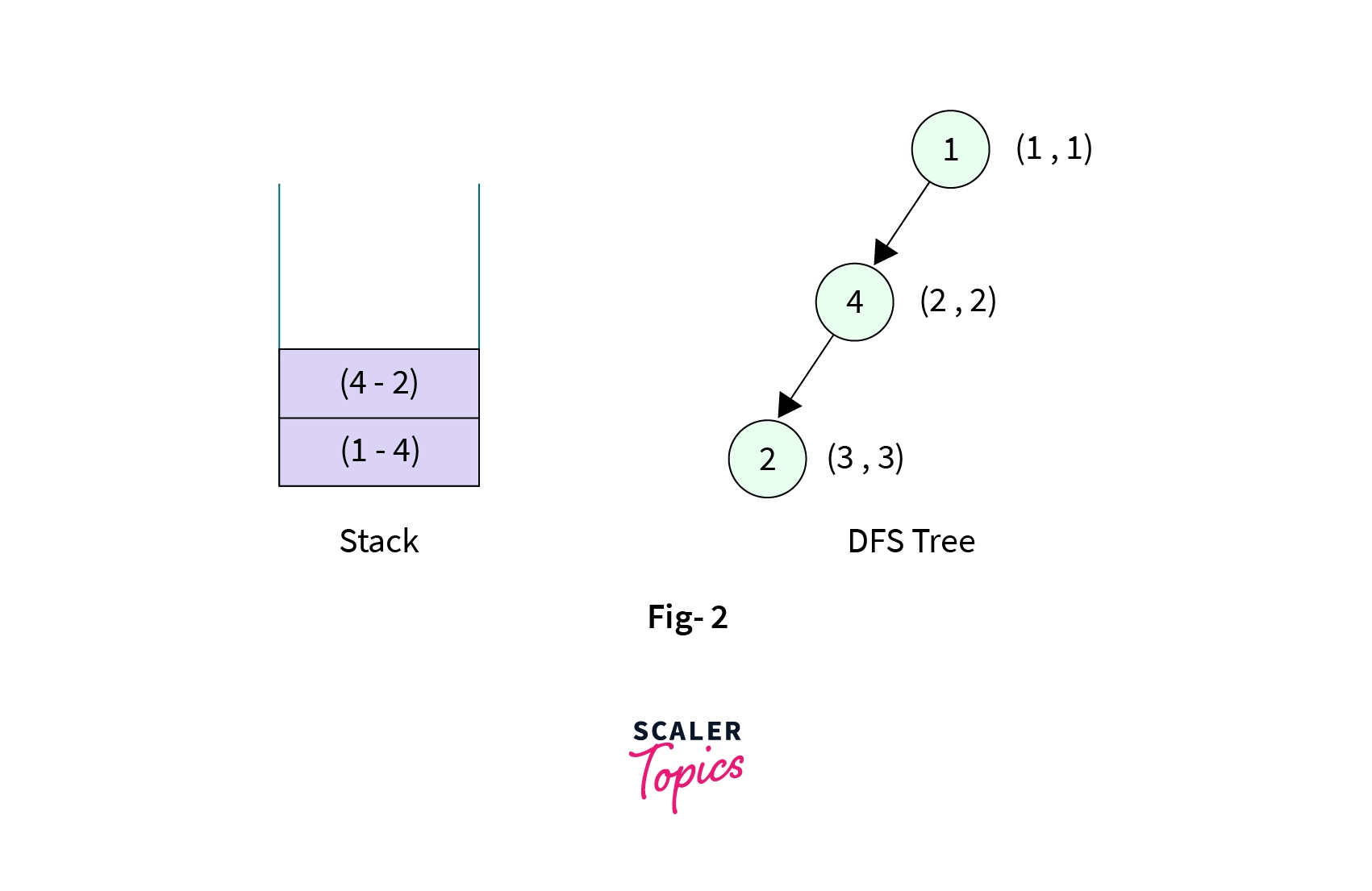
• Now the control is at the Node-4. It has two children (Node-1 and Node-2), Node-1 is already visited so we make DFS call to Node-2. Node-2 is then marked visited with discovery time and low time as (3, 3) and the edge from Node-4 to Node-2 is pushed onto the stack. The stack now contains two elements,

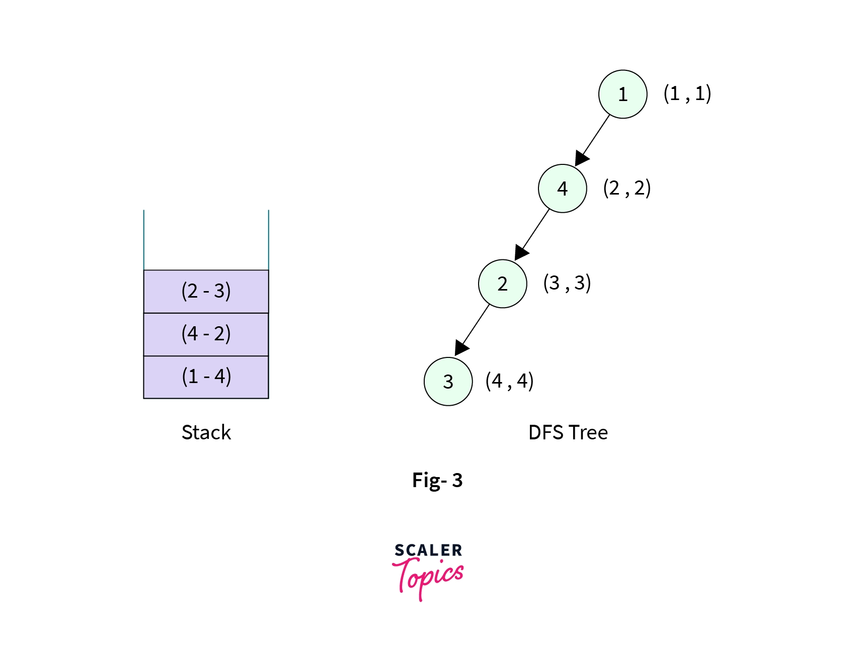
• Now the control is at the Node-2. It has four children (Node-4, Node-3, Node-5 and Node-6), Node-4 is already visited and is the parent of Node-2 so we make DFS call to Node-3. Node-3 is then marked visited with discovery time and low time as (4, 4), and the edge from Node-2 to Node-3 is pushed into the stack. The stack now contains three elements,

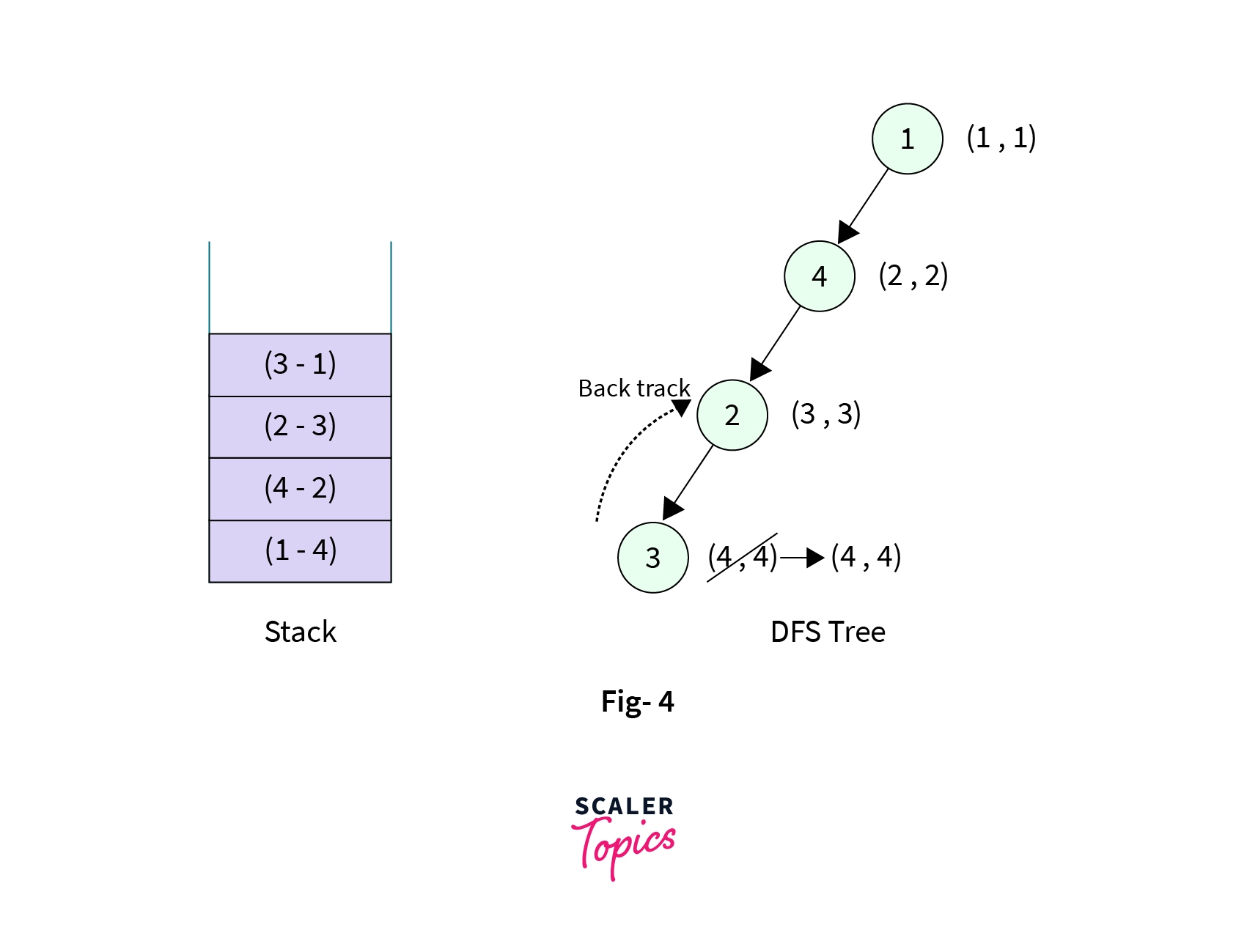
• Now the control is at the node Node-3. It has two children (Node-1 and Node-2), both of the children are visited but Node-1 is not the parent node for Node-3, so we add the edge from Node-3 to Node-1 into the stack and backtrack to Node-2. Also, we assign a new low[] value to Node-3 that is the low[] value of node Node-1 as Node-1 is already visited and not the parent node of Node-3. The stack now contains four elements,

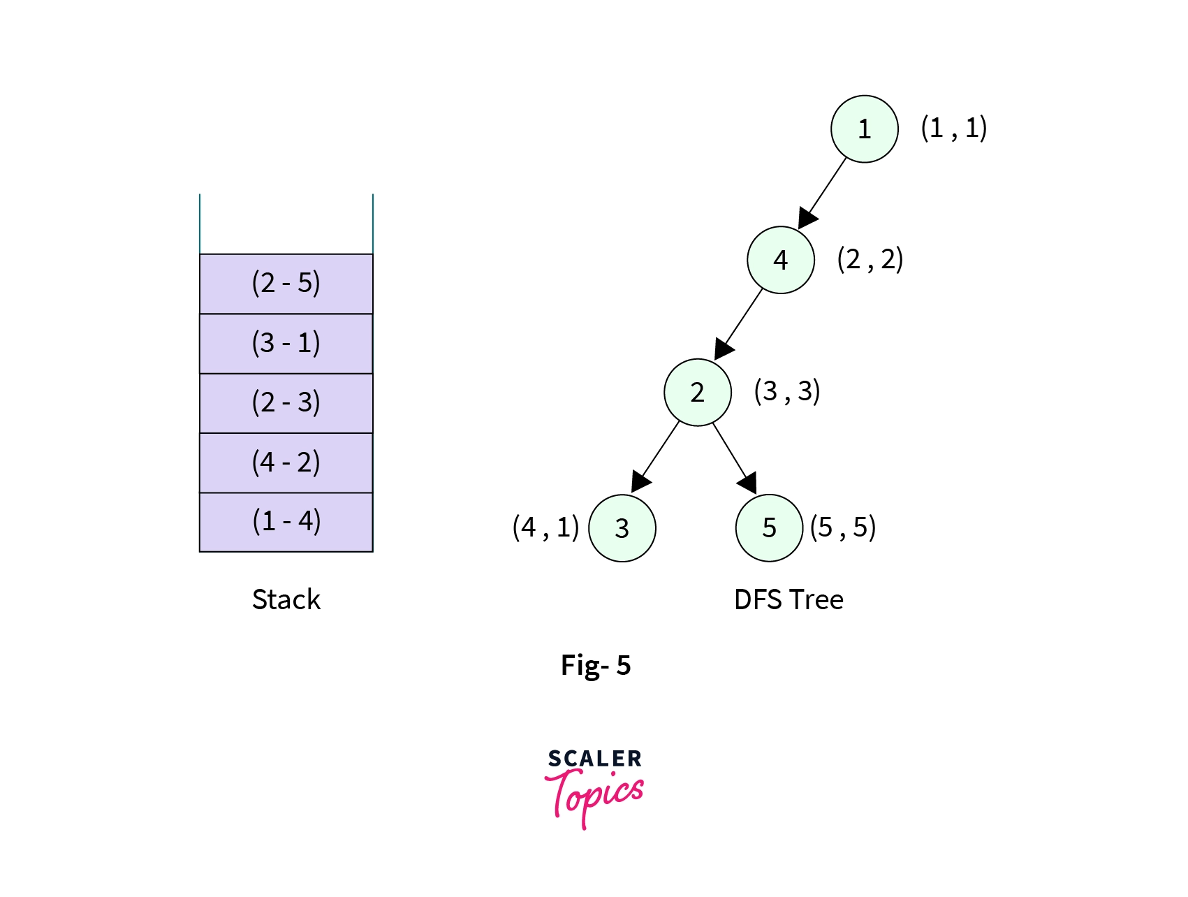
• Now we are again at Node-2, we make DFS call to its child Node-5 as it is unvisited. Node-5 is then marked visited with discovery time and low time as (5, 5). Also, the edge from Node-2 to Node-5 is pushed into the stack. Stack now contains 5 elements,

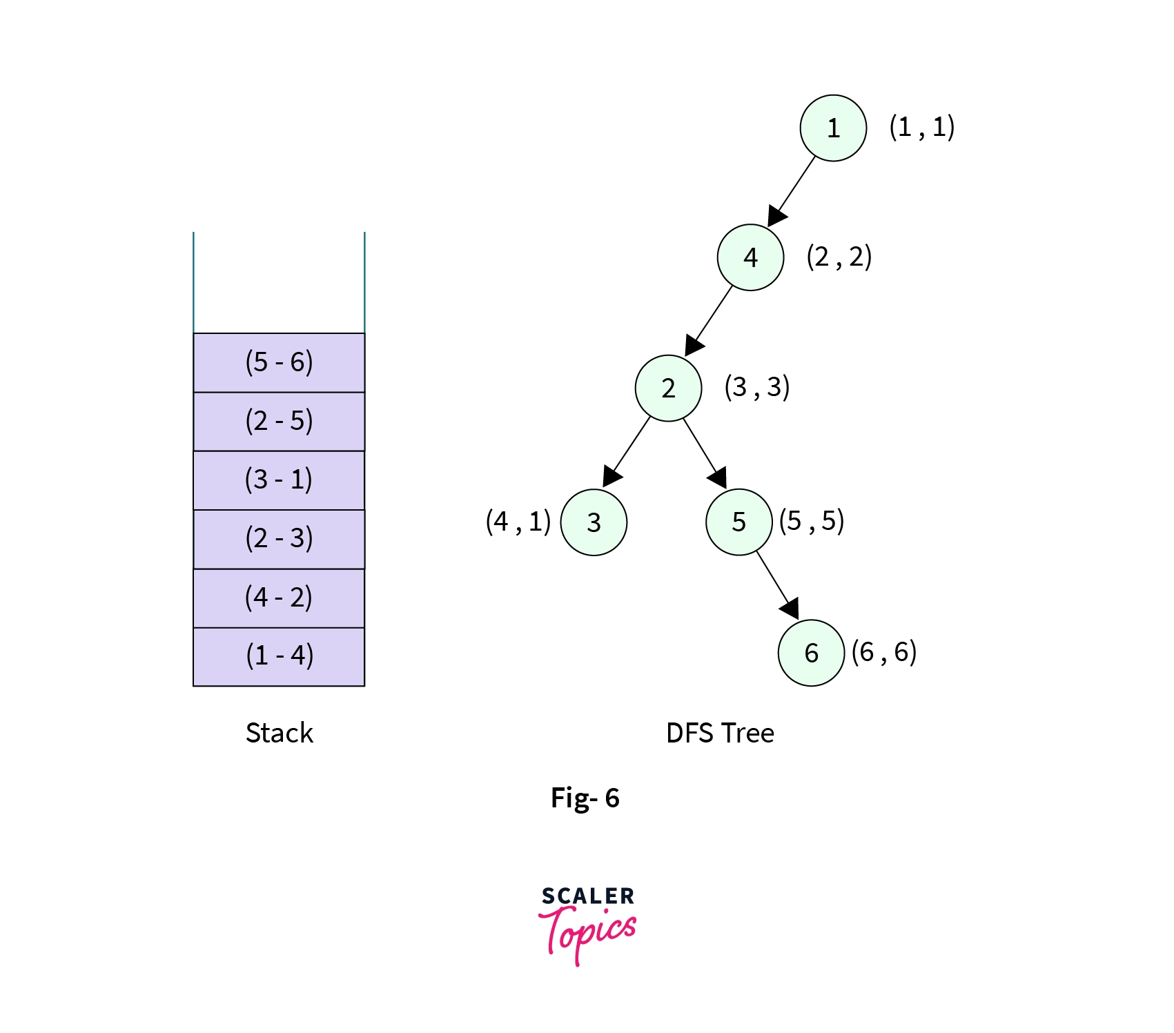
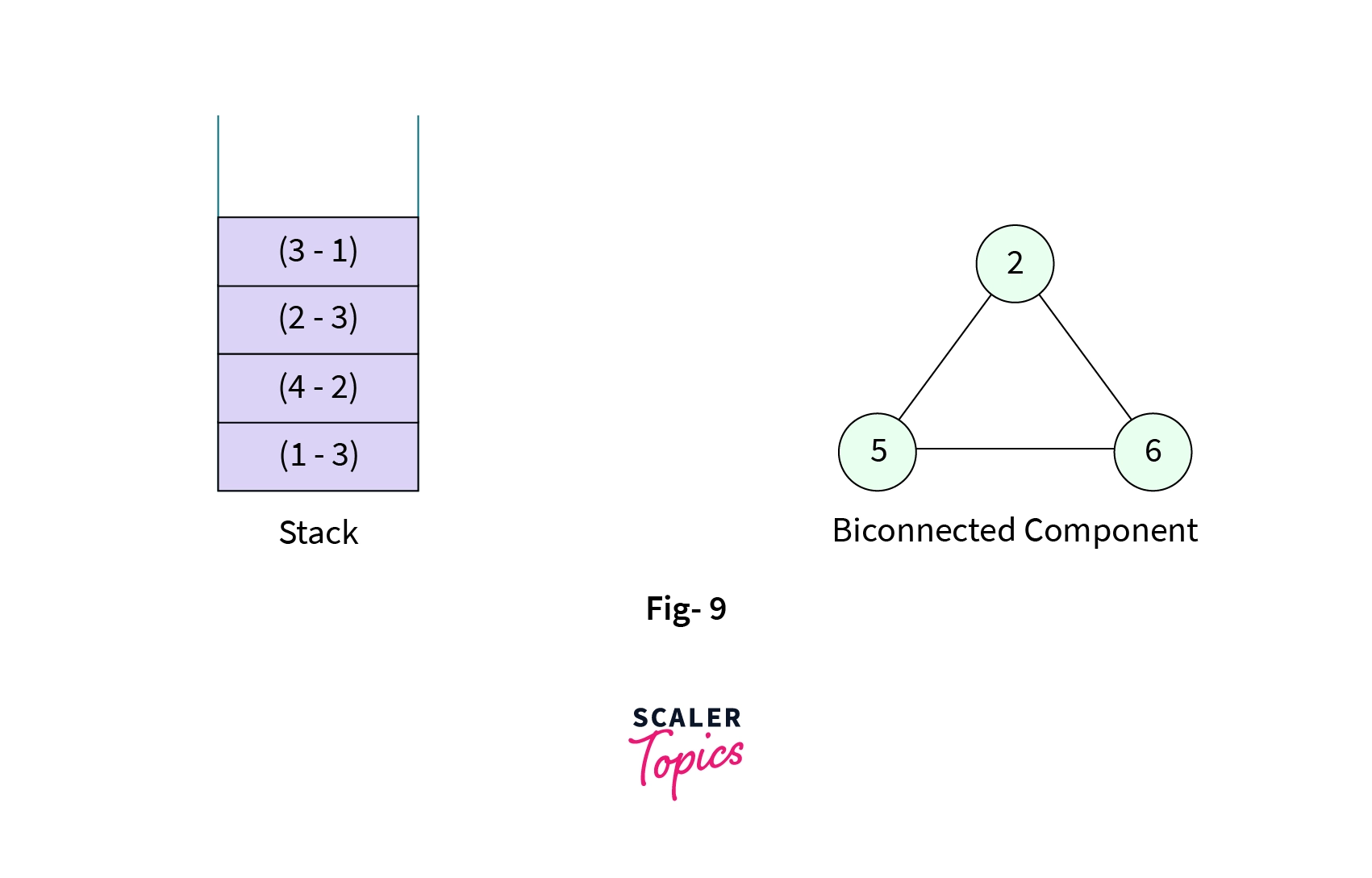
• Control is at Node-5, it has two children (Node-2 and Node-5), Node-2 is the parent and already visited we have no business to do there. DFS call is then made to Node-6 it is marked visited with discovery time and low values as (6, 6) and the edge from Node-5 to Node-6 is added to the stack. Stack now contains six elements,

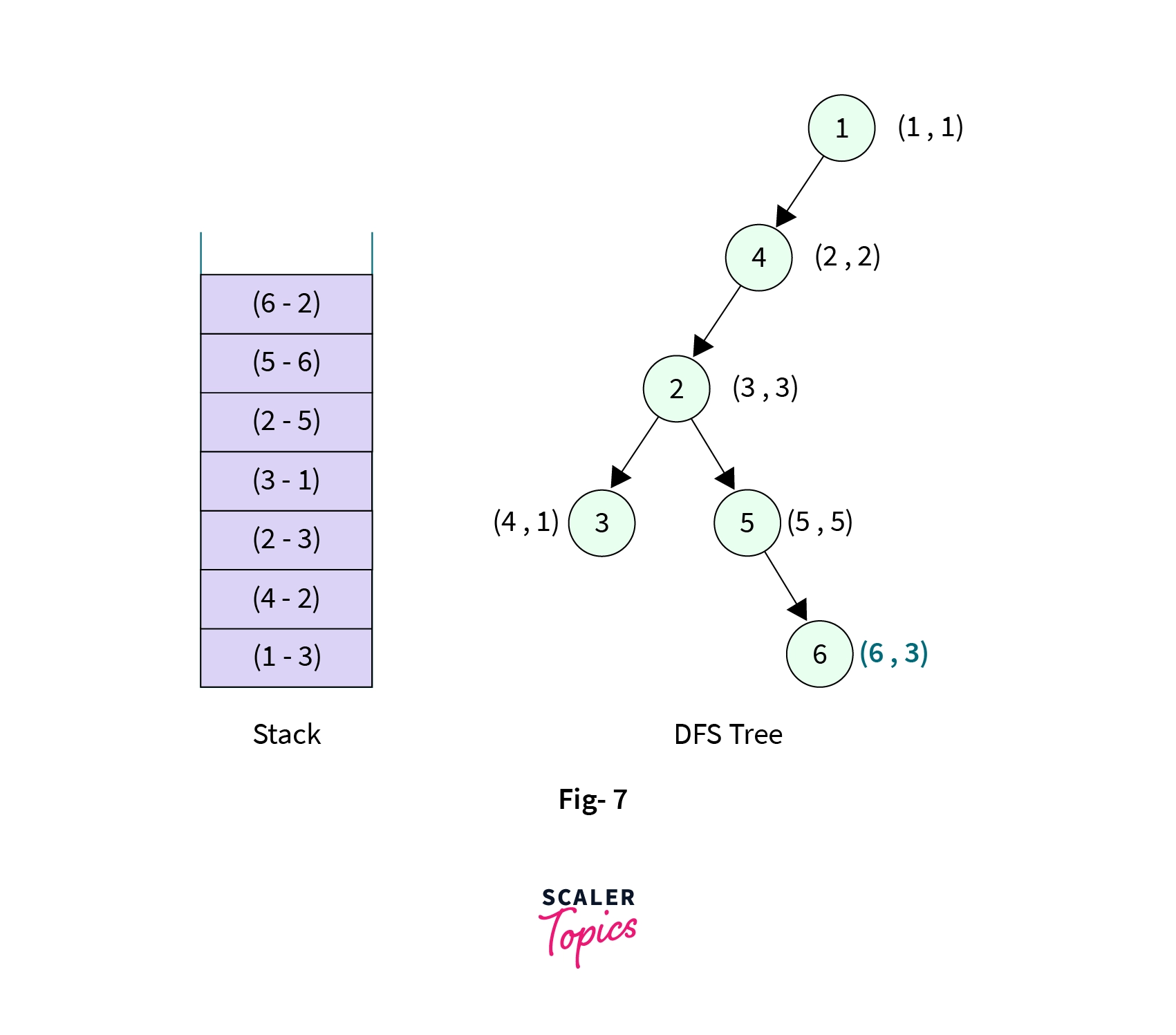
• Now the control is at Node-6, it has two children(Node-2 and Node-5). Node-5 is the parent node and already visited but Node-2 is not the parent node but it is already visited, so we mark the low value of Node-6 to discovery value of Node-2 that is low[6] = disc[2] => 3. We also add the edge from Node-6 to Node-2 into the stack. Stack now contains seven elements,

• Now all the children of Node-6 are visited, we then backtrack to Node-5, here we see that the child Node-6 of Node-5 have less low[] value than the Node-6. We update the low[] value of Node-5 to low[] value of Node-6. That is, low[5] = low[6] => 3.

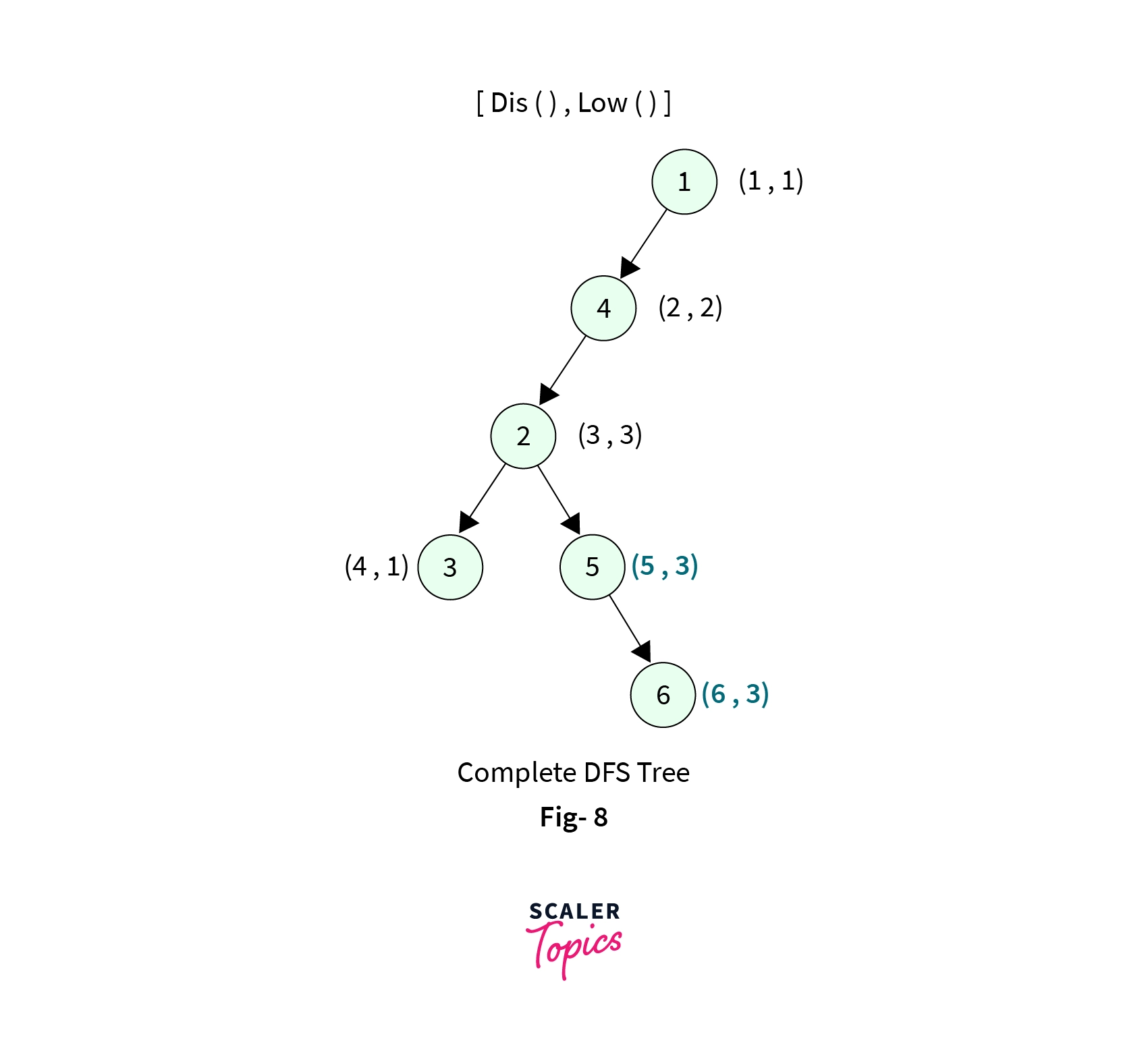
• Now we backtrack to Node-2, this is the moment where we print out first biconnected component. Since low[5] >= disc[2], which is indeed a condition for Articulation point. We print the elements of the stack until we reach the edge (2-5). This pops 3 elements from the stack and forms a connected component shown below,

• When all the nodes are visited starting from the source node DFS call return to the source node and finally the 4 elements left in the stack form another Biconnected component. The two Biconnected components in the graph are shown below,

Implementation of Biconnected Components in C++

• In the main function, we take input of the number of nodes(n) and the number of edges(m) in the graph. After that, we create the adjacency list to represent the graph. Once we are done with the input work, we create an object of class Solution.
• This sol object has access to a public method of class Solution print_biconnected_component(). We simply call this method passing the graph and the number of nodes. The rest is the same as discussed in the algorithm above.

Implementation of Biconnected Components in Java

Implementation of Biconnected Components in C#

Output -

• Time Complexity : We are doing no fancy work except the Depth first Search. So the time complexity of this program will be O(V + E), where V is the number of nodes and E is the number of edges. Which is same as the time complexity of Depth first search.
• Space Complexity : We are using total 5 arrays here namely vis, disc, low, graph, par. So the space complexity is O(5 * N). We also need a O(N) recursion stack space to make DFS calls. N is the number of nodes in the graph.