Ford-Fulkerson Algorithm for Maximum Flow Problem

Introduction

If we consider a rail network that connects two cities (say $A$ and $B$) by way of several intermediate cities, where each railway line has some value assigned to it denoting its capacity.

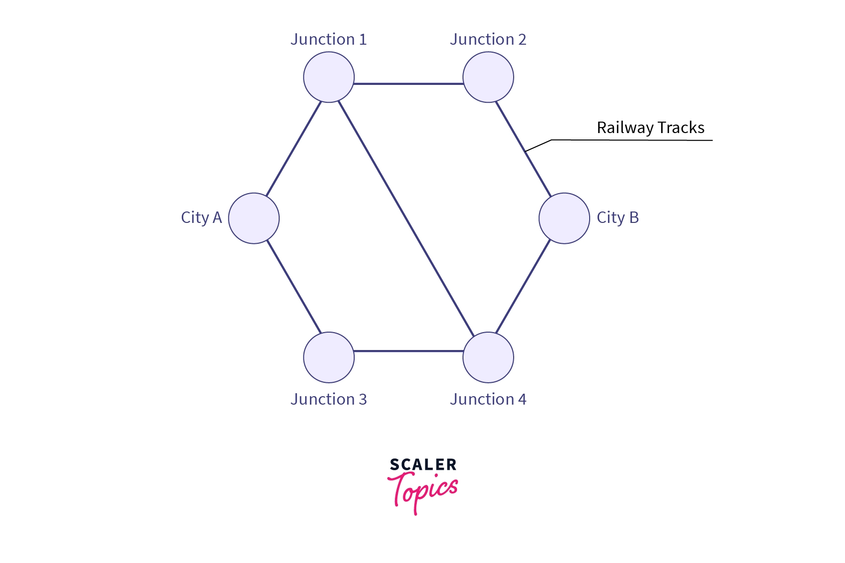
Flow can be defined as any physical/virtual thing that we can transmit between two vertices through an edge in a graph, for example - water, current, data and in this case "trains".

Assuming steady conditions (Number of trains on a railway track at any instance of time must not exceeds the track's capacity), if we need to find what is the maximum number of trains (maximum flow) that we can send from City $A$ to city $B$ then the problem is known as the "Maximum Flow Problem". Before introducing the problem formally firstly let's have a look at some terminologies for a better understanding of the problem and its solution.

Flow Network

In graph theory, a flow network is defined as directed graph $G=(V,E)$ constrained with a function $c$, which bounds each edge $e$ with a non-negative integer value which is known as $capacity$ of the edge $e$ with two additional vertices defined as source $S$ and sink $T$.

As shown in the flow network given below, a source vertex has all outgoing edges and no incoming edges, more formally we can say In_degree[source]=0 and sink vertex has all incoming edges and no outgoing edge more formally out_degree[sink]=0.

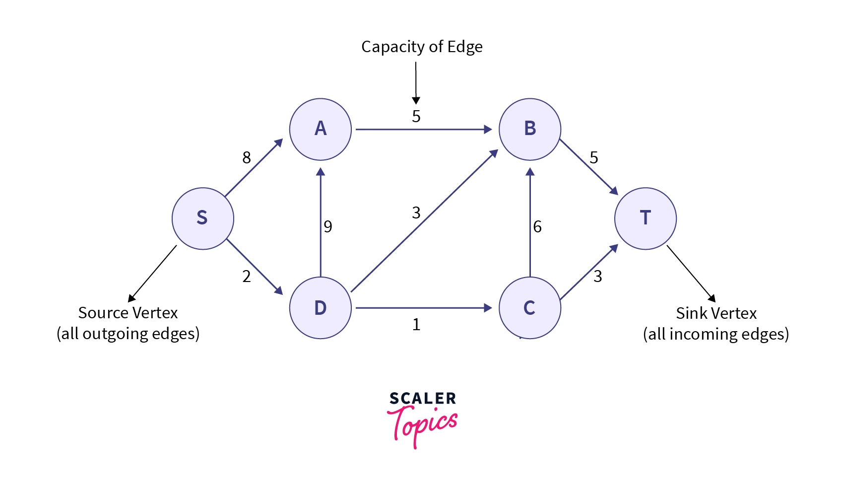
Also, any flow network should satisfy all the underlying conditions --

• For all the vertices (except the source and the sink vertex), input flow must be equal to output flow.
• For any given edge($E_i$) in the flow network, 0$\leq flow(E_i)\leq capacity(E_i)$ must hold, we can not send more flow through an edge than its capacity.
• Total outflow from the source vertex must be equal to total inflow to the sink vertex.

Maximum Flow Problem Introduction

The underlying image represents a flow network, where the first value of each edge represents the amount of the flow through it (which is initially set to 0) and the second value represents the capacity of the edge.

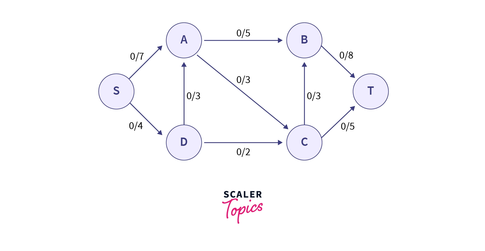
The maximum flow is the maximal possible value of the flow of the network where the flow is defined as, "sum of all the flow that gets produced in source $s$, or sum of all the flow that gets consumed in the sink $t$ ".

If we try to co-relate this problem with a real-life problem, we can visualize all the edges as water pipes, where the capacity of edge (here pipe) is the maximum amount of water that can flow through it per unit time. Where $s$ is analogous to the Water plant and $t$ is analogous to the drainage plant.

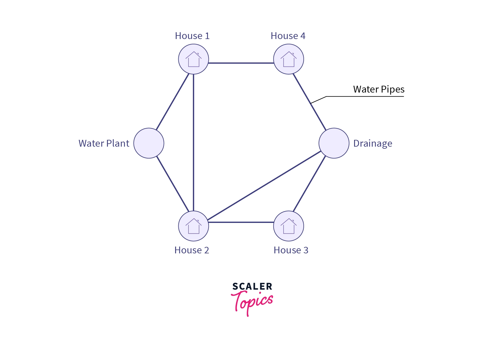
It follows the conditions necessary for a flow network that more water than pipe's capacity can't flow through it and water inflow and outflow of water at every vertex (house) must be equal as water can't magically disappear or appear.

Formally, Maximum flow can be defined as -

A Naive Greedy Algorithm

The naive approach that comes to our mind is a greedy algorithm that involves finding a path from the source node ($s$) to the sink node ($t$) and if the path exists then increasing the flow as much as possible such that along any edge do not exceed its capacity.

Let's look at the algorithm -

E = number of the edges in the flow network. $f(e)$ = flow along the edge edge $e$. $c(e)$ = Capacity of the edge $e$.

• Initialize the maxFlow with 0 $i.e.$ maxFlow=0
• Use BFS/DFS to search for a path between the vertices $s$ and $t$. Here existence of path $P$ means, for every edge $e$ in $P$, $f(e) < c(e)$ must hold. If such a path exists then -
  • flowCanBeAdded = $min(c(e)-f(e))$ for each edge $e$ in $P$.
  • maxFlow = maxFlow + flowCanBeAdded
  • For each edge $e$ in $P$, $f(e)=f(e)+$flowCanBeAdded
• In the other case (There does not exist any path between $s$ and $t$) return the maxFlow.

Let's try the above algorithm on the underlying flow network -

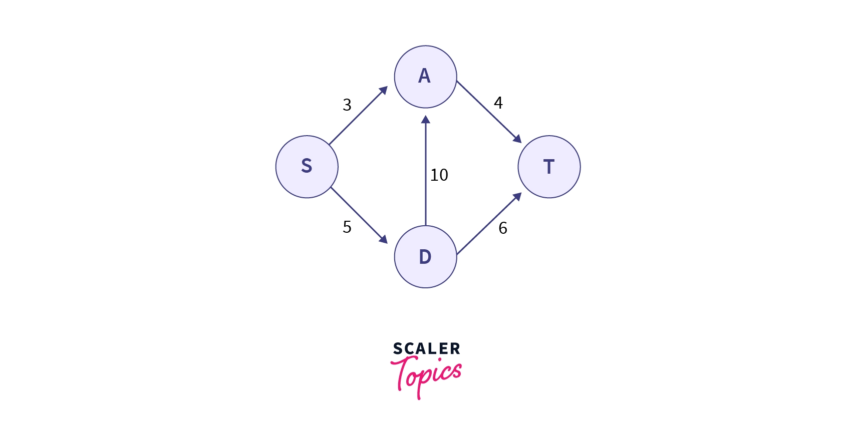
According to the algorithm, in the above flow network, we will search for a path between $s$ and $t$. Let's assume we choose the path $s\rightarrow B \rightarrow A \rightarrow t$ with capacities as $5, 10, 4$. The minimum among them is $4$, so we will increase that much flow along the path, after which our flow network will look like -

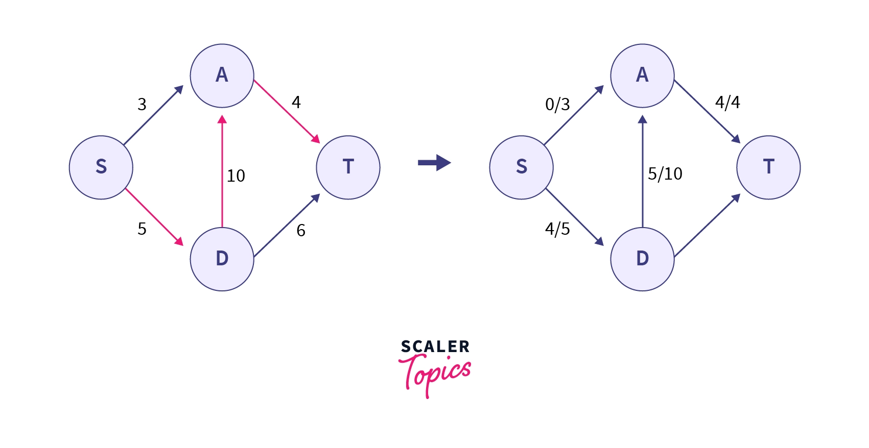
Now we are not left with any other valid path between $s$ and $t$ so according to the algorithm, the maximum flow is $4$.

But, it is easily noticeable that the maximum flow that can be obtained is $8$ by choosing the paths $s\rightarrow A \rightarrow t$ and $s\rightarrow B \rightarrow t$. So we can say that the greedy algorithm doesn't give the correct answer always. To obviate this difficulty we use the Ford-Fulkerson method that uses the concept of residual graph which has been discussed in detail in the next section.

Ford-Fulkerson Algorithm for finding Maximum Flow

This algorithm was developed by L.R. Ford and Dr. R. Fulkerson in 1956. Before diving deep into the algorithms let's define two more things for better understanding at later stages -

• Residual Capacity - Residual capacity of the directed edge is nothing but capacity of the edge - current flow through the edge. If there is flow along a directed edge u → v then reversed edge has a capacity 0 and we can say $f(v,u)=-f(u,v)$
• Residual Graph - Residual graph is nothing but the same graph with the only difference is we use residual capacities as capacities.
• Augmenting Path - It is a simple path from source to sink in a residual graph i.e. along the edges whose capacity is $0$.

In the Ford-Fulkerson method, firstly we set the flow of each edge $e$ to $0$. Then we look if an augmenting path exists between $s$ and $t$. If such a path exists then we will increase the flow along those edges.

We repeat this process until there is at least on more augmenting path in the residual graph. Once there are no more augmenting paths maximal flow is achieved.

Let us see what does increasing the flow along an augmenting path means. Let $X$ be the minimum residual capacity found among the edges of augmenting path.

Then, for every edge $(u, v)$ in the path we do $f(u,v)+=X$ (Forward edges) and $f(v, u)-=X$ (backward edges).

Now we use the above network to demonstrate how the Ford-Fulkerson method works.

Example

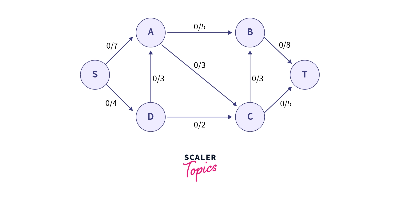
We can see that the initial flow of all the paths is $0$. Now we will search for an augmenting path in the network.

One such path is $s \rightarrow A \rightarrow B \rightarrow t$ with residual capacities as $7$, $5$, and $8$. Their minimum is $5$, so as per the Ford-Fulkerson method we will increase a flow of $5$ along the path.

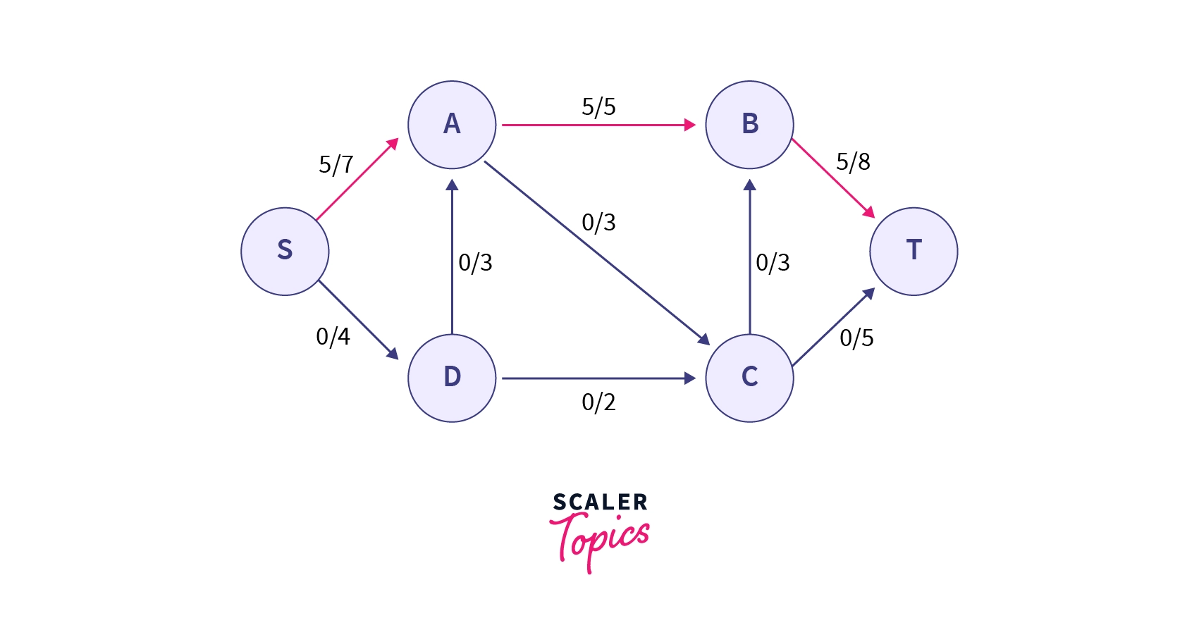
Now, we will check for other possible augmenting paths, one such path can be $s \rightarrow D\rightarrow C\rightarrow t$ with residual capacities as $4$, $2$, and $5$ of which $2$ is the minimum. So we will increase a flow of $2$ along the path.

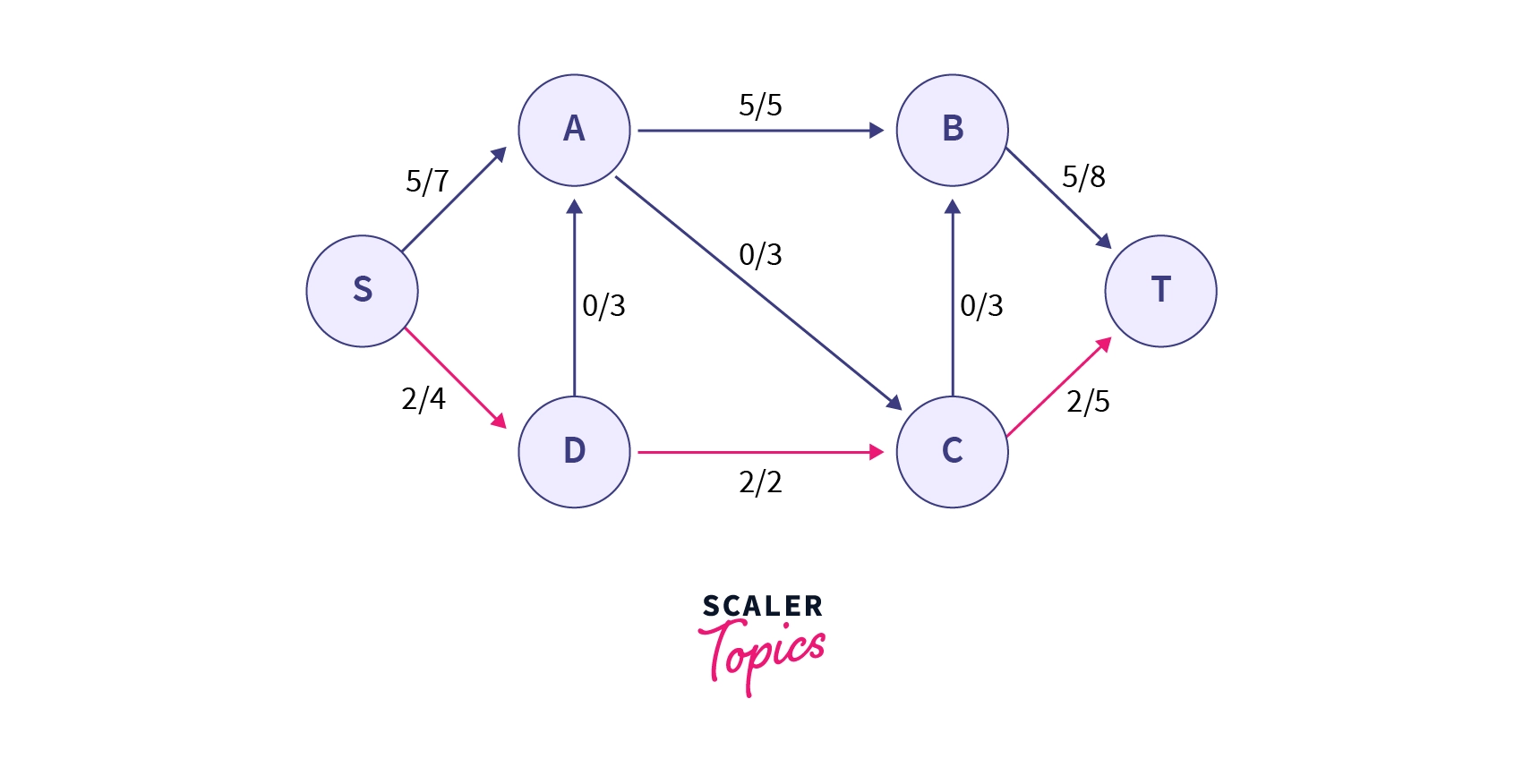
One can easily observe from the figure that we can't increase the flow along paths $A \rightarrow B$ and $D \rightarrow C$ as their flow has reached their maximum capacity. So to find other augmenting paths, we must take care that these edges must not be part of the path.

One such path can be $s\rightarrow D \rightarrow A\rightarrow C \rightarrow t with residual capacities as$2$,$3$,$3$, and$3$of which$2$is the minimum so will increase a flow of$2$ along the path.

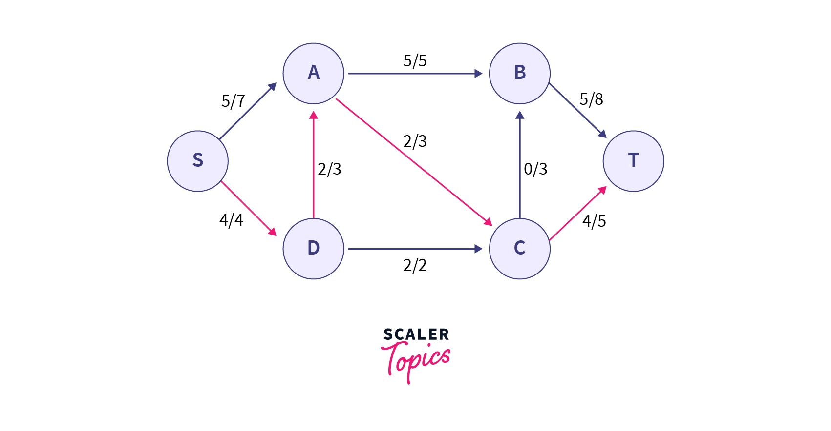
An augmenting path that is possible in the current residual network is $s\rightarrow A \rightarrow C \rightarrow t$ with residual capacities as $2$, $1$, and $1$ of which $1$ is minimum.

So we will increase the flow of $1$ along the path after which our network will look like -

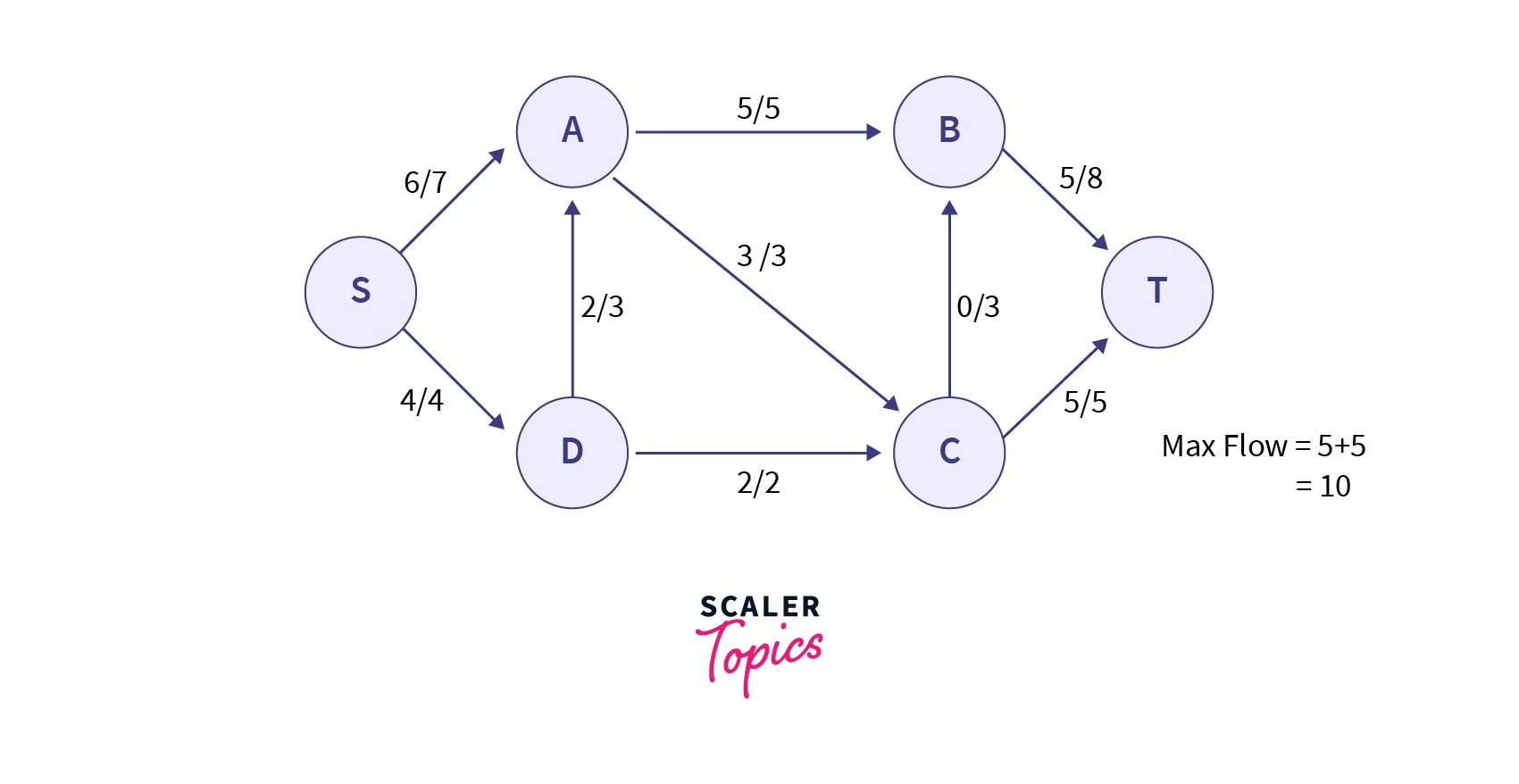
Now there are no more augmenting paths possible in the network, so the maximum flow is the total flow going out of source or total flow coming in sink i.e. $6+4=5+5=10$

Pseudocode

Code

To keep things simple, we are using adjacency matrix implementation of the graph. The flow of writing code will be -

• Making a residual graph from the values of the given graph.
• Declaring a parent array of size $V$ to store the augmenting path during BFS.
• Finding the bottle-neck capacity (minimum residual capacity) of the augmenting path.
• Updating residual capacities of edges and reverse edges.
• Increasing the overall path flow.
• Returning answer i.e. maximum flow.

C/C++ implementation of Ford-Fulkerson Method

Java implementation of Ford-Fulkerson Method

Complexity Analysis

The above implementation of the Ford-Fulkerson algorithm is called Edmonds-Karp Algorithm. The idea of Edmonds-Karp is to use BFS to find the augmenting path in the residual network.

Because we can implement each iteration of the Ford-Fulkerson Method in $O(E)$. As we use BFS to find augmenting path (Edmonds-Karp implementation) overall time complexity would be $O(V*E^2)$ in the worst case. Since, Adajency Matrix representation of the graph is used in the above implementation therefore, BFS would take $O(V^2)$ time, and hence the overall time complexity is $O(E*V^3)$.

Applications.

• In traffic movements, to find how much traffic can move from a City $A$ to City $B$.
• In electrical systems, to find the maximum current that could flow the wires without causing any short circuit.
• In the water/sewage management system, to find maximum capacity of the network.