Hamiltonian Path

Introduction to Hamiltonian Path

• Hamiltonian Path is just a permutation of all vertices of a connected graph component.
• A Hamiltonian Cycle is also a Hamiltonian Path but with the same ending and starting vertices.

In most of the real-world problems, one may encounter a lot of instances of the Hamiltonian Path problem for example: Suppose Ray is planning to visit all houses in his neighborhood this Christmas and to save his time he wants to walk on such a path that he visits each house exactly once and he does not have to encounter the already visited house again in the path he has taken, refer the image below for the above scenario

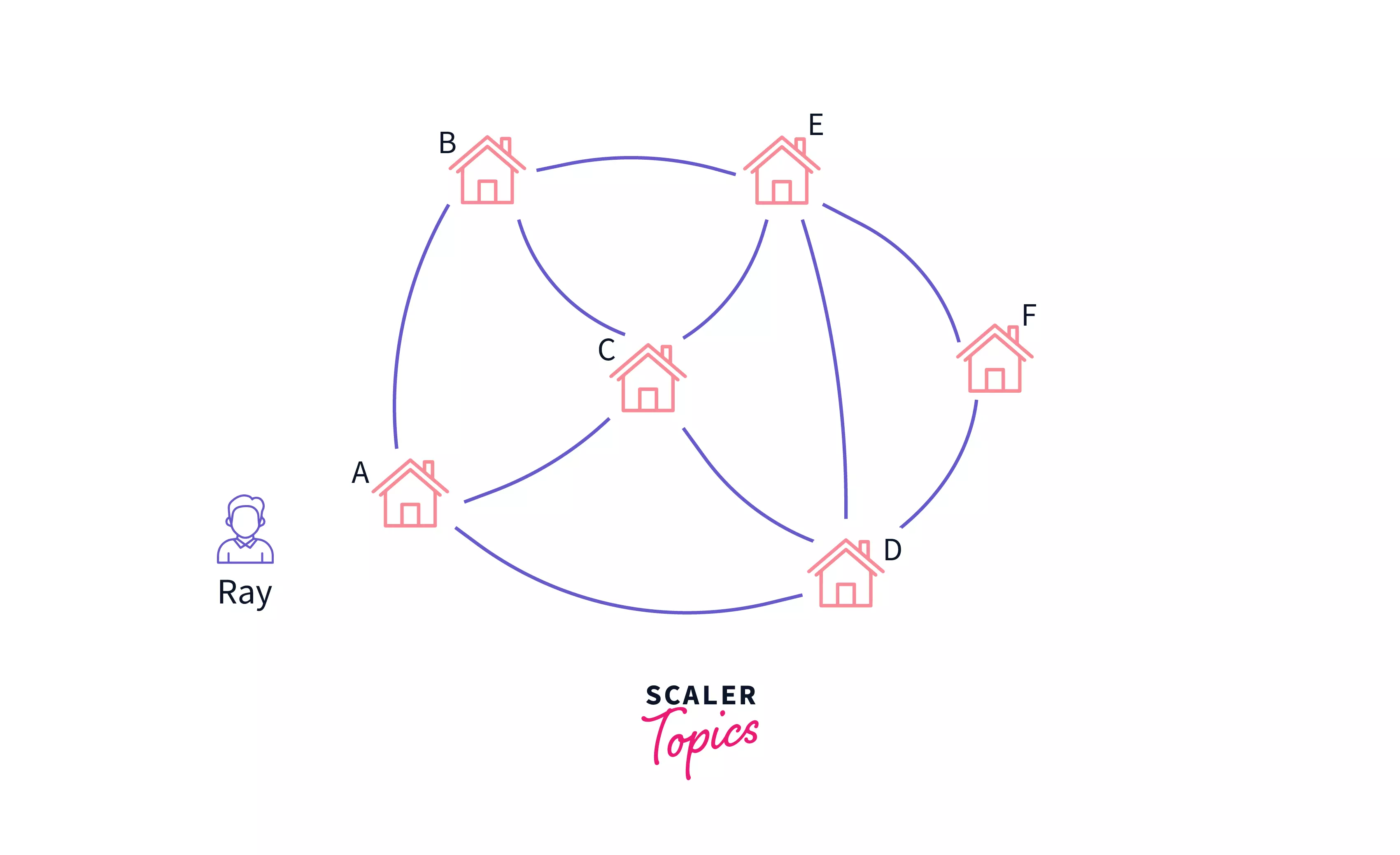
In the above figure, A, B, C, D, E, F represents the houses of Ray's neighbors where he wants to visit, the blue bold lines represent the direct street from one house to another and there are nine such streets each connecting a different pair of houses i.e. there is at most one street between two houses in this example but in the general case, there can be multiple as well, and he is starting to visit from house A.

Try to figure out a path starting at A and visiting all houses i.e. A, B, C, D, E, F exactly once, Ray takes the path as shown below

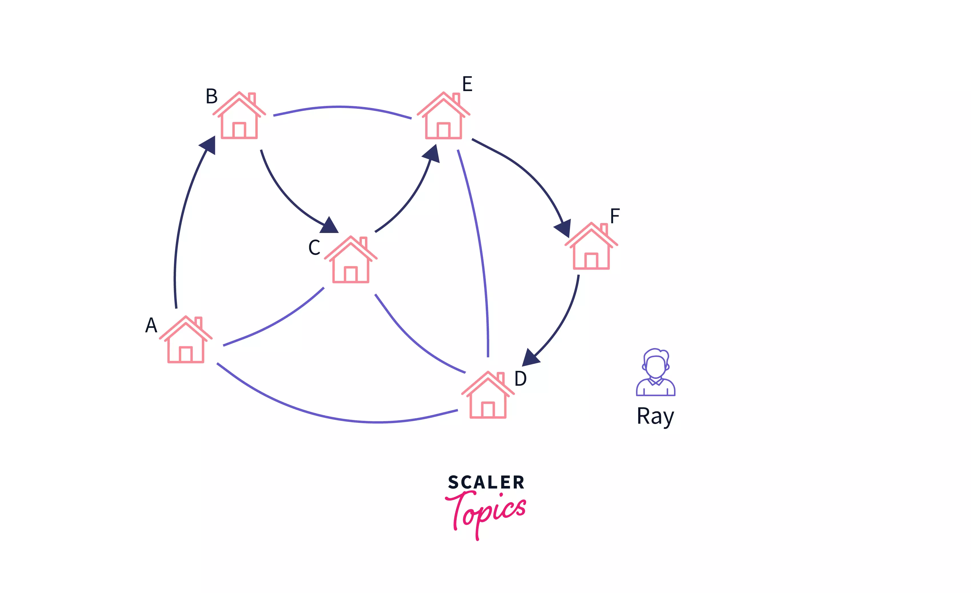
The path is A->B->C->E->F->D, and it visits every house exactly once and finally Ray is able to visit all houses in the minimum walk or we can say time also it is obvious that there are more than one such paths that visit all houses exactly once (try enumerating all such paths).

The paths that we obtained here are called hamiltonian paths and such paths exist in connected graphs, let's jump to the formal definition of Hamiltonian Path.

Definition of Hamiltonian Path

• Hamiltonian path in a connected graph is a path that visits each vertex of the graph exactly once, it is also called traceable path and such a graph is called traceable graph, Hamiltonian Path exists in directed as well as undirected graphs.
• There can be more than one Hamiltonian path in a single graph but the graph must be connected to have the possibility of the existence of a Hamiltonian path.
• A graph is called Hamiltonian connected graph when there exists a Hamiltonian path between any two vertices of the graph. Refer to the image below

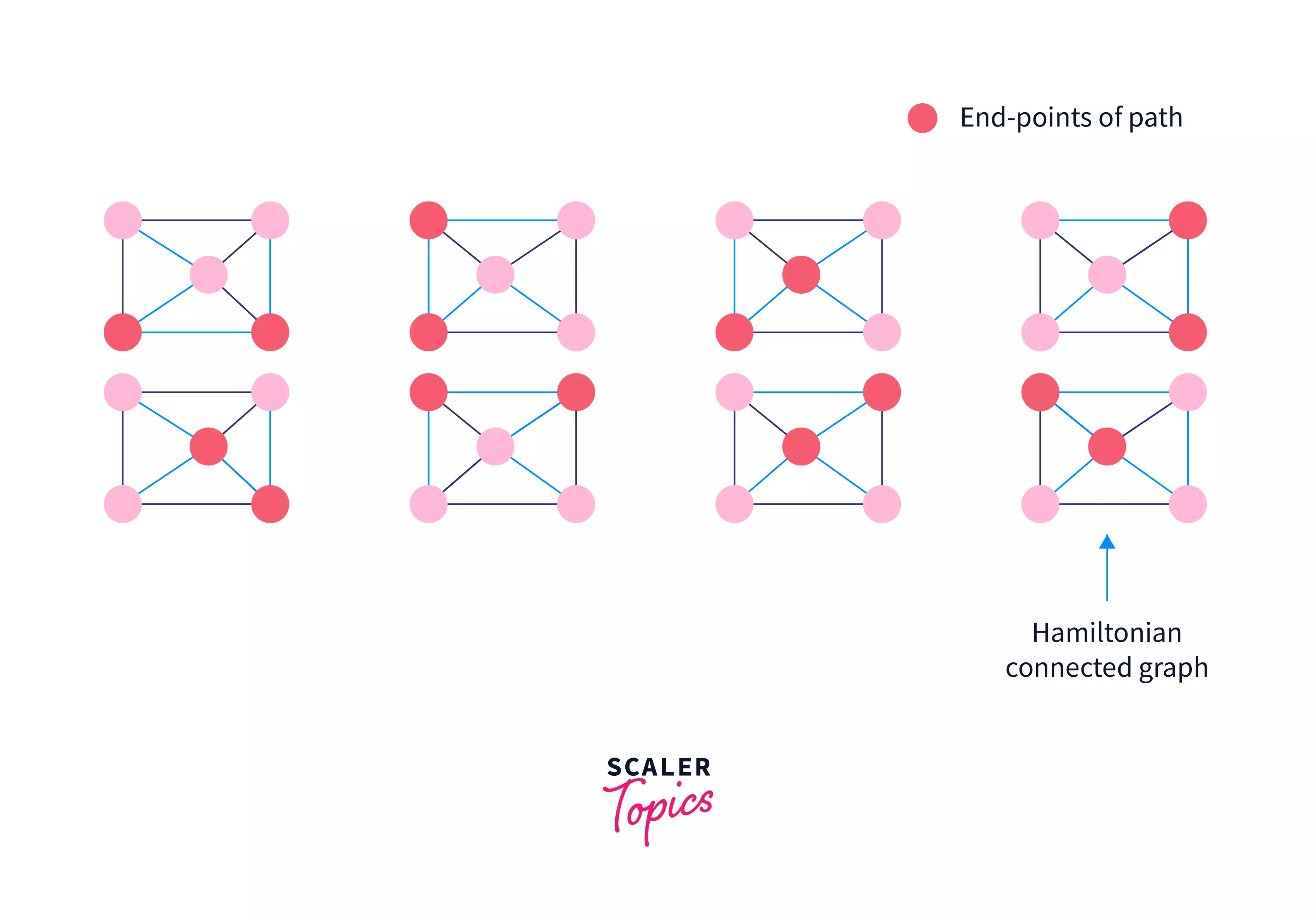
In the above figure, every pair of vertices has a Hamiltonian path between them.

• If the endpoints of the Hamiltonian path are adjacent i.e. have a direct edge between them, then those endpoints can be extended to form a Hamiltonian Cycle, where we visit each vertex in a connected graph exactly once and ends up at the same vertex where we started. Refer the image below

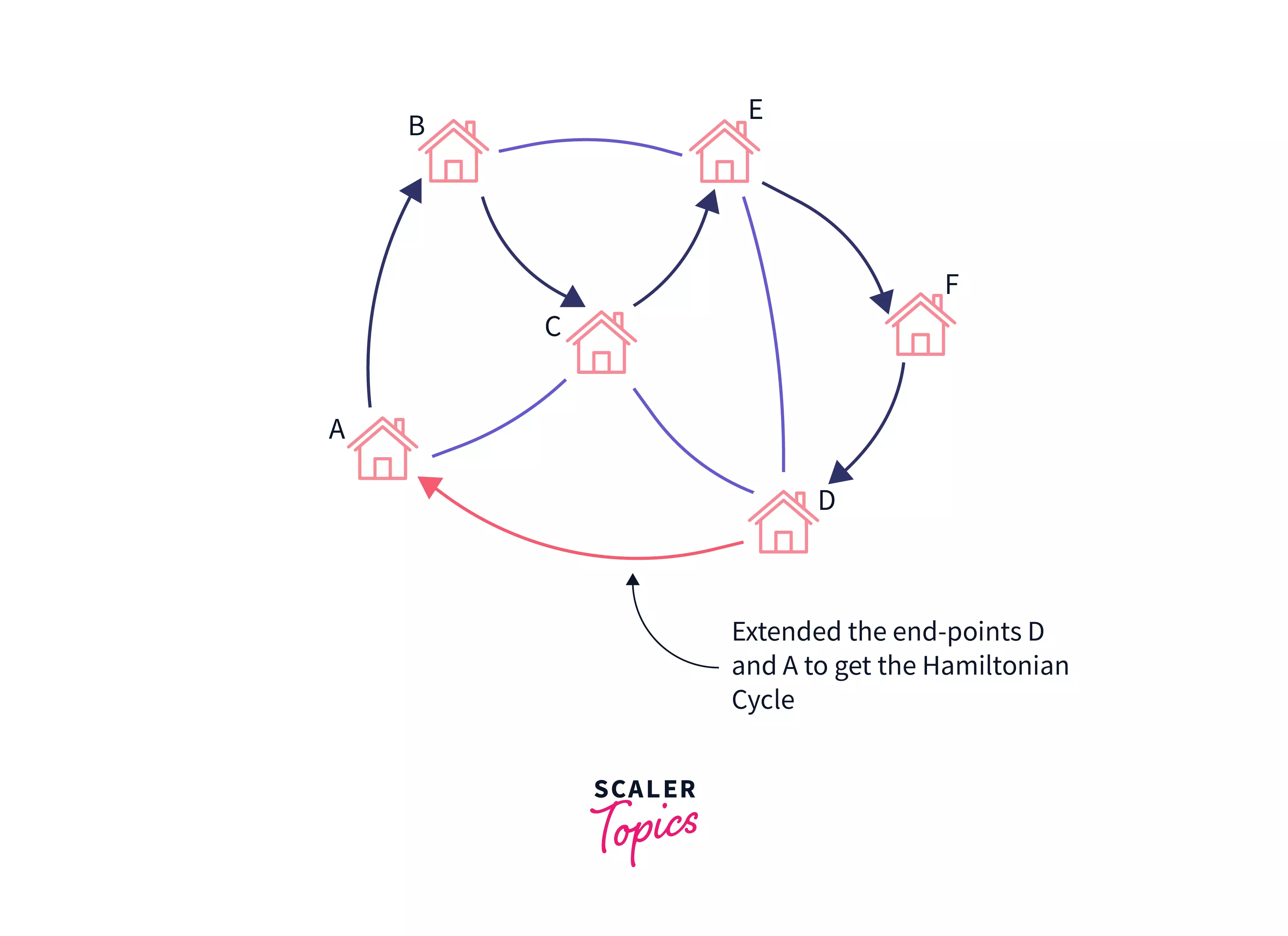
Therefore, in the figure above A->B->C->E->F->D->A represents the Hamiltonian cycle.

Ways to Check for the Existence of Hamiltonian Path in a Graph

• There is a requirement of selecting some of the permutations of vertices which are Hamiltonian Paths.
• A lot of redundant work is done in naive- algorithm for Hamiltonian Path.
• Dynamic programming approach takes $O(N^2 * 2^N)$.
• Depth-first Search is also used for checking Hamiltonian Path in a connected graph with $O(N!)$ worst-case time complexity.

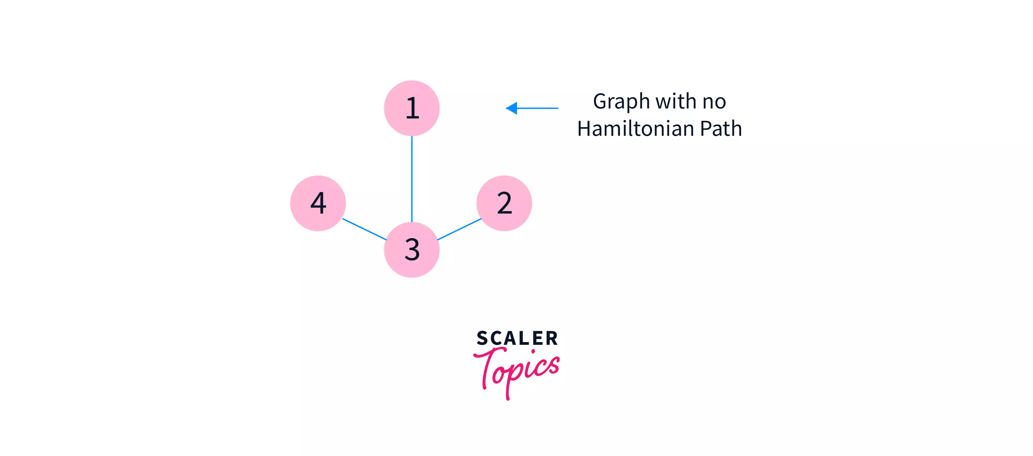
Let's think about the different ways in which the Hamiltonian Path can be detected in a graph because it is obvious that there can be graphs where there is no Hamiltonian Path at all (think about such graph) for example disconnected graph i,e, graph having more than one connected component or another graph as shown in the image below. Therefore, we need some techniques that can be used to check whether a Hamiltonian Path exists in a graph or not.

Let's jump into the process of building an algorithm to check for the Hamiltonian Path. Think about a Hamiltonian Path as it’s just a sequence of all vertices of the graph where each vertex appears exactly once, so this drives us to the conclusion that for a graph having 4 vertices numbered from 1 to 4, the Hamiltonian Path will be a permutation of those four vertices where any two adjacent vertices in the permutation have a direct edge as shown in the image below

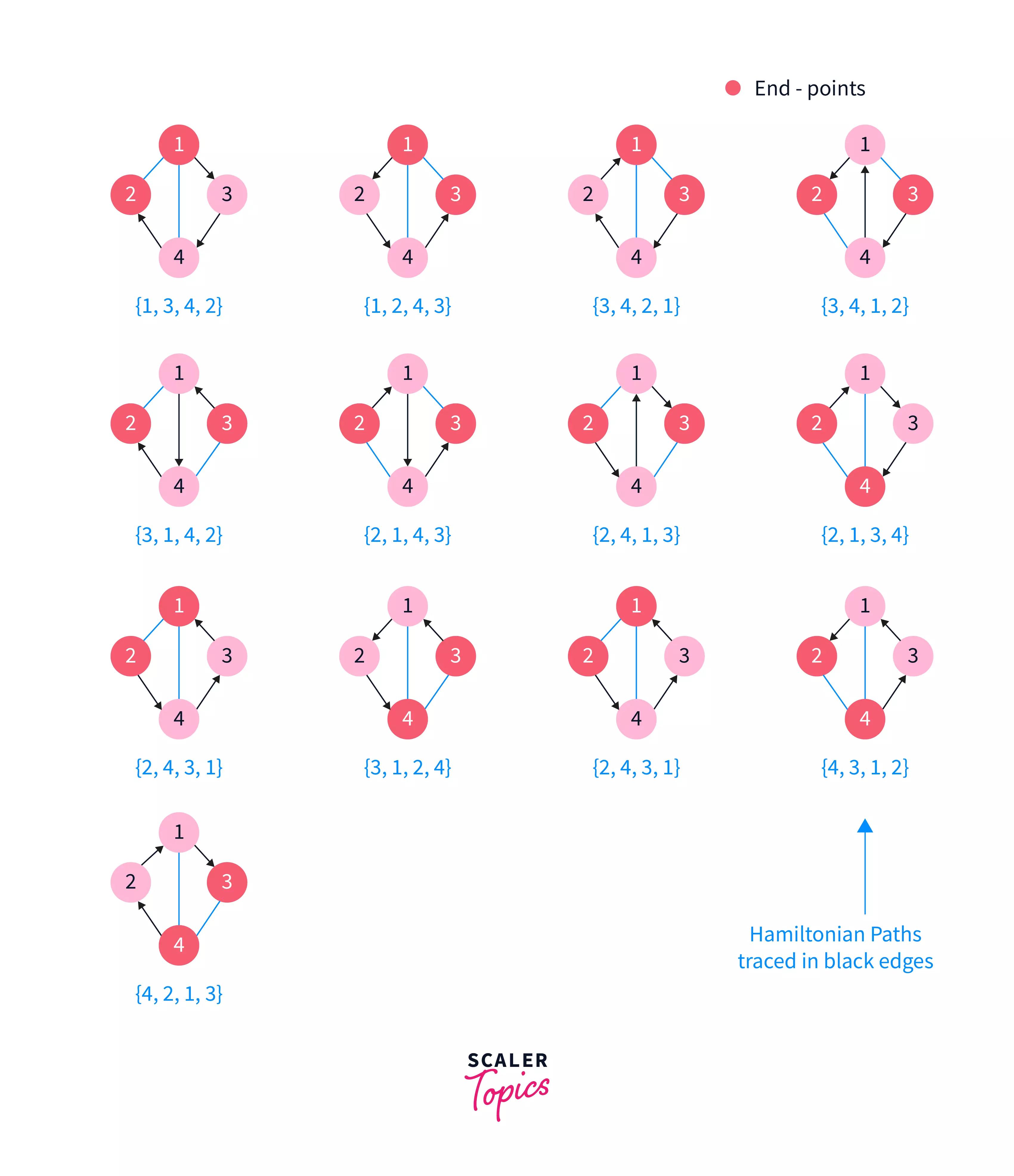
In any of the Hamiltonian Paths shown above, they are just permutations of all vertices such that any two adjacent vertices in the permutation have a direct edge between them let's take the first Hamiltonian Path that is {1,3,4,2}, we can observe that any two adjacent vertices of the permutation {1,3},{3,4},{4,2} has a direct edge between them. Let's jump to the formal definition of the approach.

1) Generating Permutations of the Vertices of the Graph G

Therefore, the first approach to check the existence of Hamiltonian Path in a connected graph having n vertices is to generate all permutations of vertices {v1,v2,v3,...,vn} and for each permutation simply check if there exists an edge between vi and vi+1 for all 1 <= i <= n-1, if it is true then this permutation of vertices is a Hamiltonian Path otherwise it is not.

Let's try to implement the above approach. To generate each permutation of n vertices {v1,v2,v3,...,vn}, we shall use a function say get_next_permutation( p ) which gives the next permutation of the vertices distinct from the ones previously generated, by next we mean the function generates permutations in lexicographically ascending order and hence we get the just next lexicographically greater permutation of p.

Hence, we start from the simplest permutation that is {1,2,3,...,n} and check if this is a valid Hamiltonian Path by linear traversal and comparing adjacent vertices for the existence of edge and then we generate the next permutation of it and check for that and so on, in this way we can generate all Hamiltonian Paths. This is the most naive and simplest approach to find Hamiltonian Path.

Let's look at the pseudocode of the above algorithm:

Pseudocode

In this function, graph in the form of adjacency matrix is passed along with n which represents the number of vertices in the graph, p is the permutation array i.e. permutation of n numbers from 1 to n, initial permutation is taken as {1,2,3,..,n}. In the while loop it basically generates all the permutations one by one and for each permutation checks if there exists an edge for every adjacent pair of vertices in that permutation, if this property is found in some permutation then that permutation is a Hamiltonian Path and we return true otherwise, it returns false.

Let's analyze the time complexity of the above approach.

Time Complexity: The get_next_permutation( p ) function generates the next lexicographical permutation by using the algorithm given by man named Narayan Pandita, it takes O(n) to generate next permutation and there are total n! permutations because each vertex is uniquely identified in the graph, Therefore the time complexity of the above algorithm is O(n*n!).

Let's look at some more optimized and subtle approaches of finding Hamiltonian Path in a connected graph.

2) Depth-first Search Approach

This is one of the naive ways of checking for Hamiltonian Path in a graph, we simply employ the property of Hamiltonian Path that is it is the path in the graph that visits every single vertex exactly once.

Using the same definition, we simply start the depth-first search from each and every vertex, and to keep track of the vertex visited we can use a visited array of size n+1 where n are the number of vertices numbered from 1 to n and initialize it with 0 means all vertices are unvisited when a vertex is visited we turn it to 1.

Also, we keep track of vertex count i.e. a number of vertices visited so far, and when it becomes equal to n that means all vertices have been visited exactly once and we return true. Vertex count is 1 while starting the depth-first search from each vertex.

If no such path is found that means there does not exist any Hamiltonian Path, hence we return false.

Let's look at the Pseudocode implementation of the above approach:

In the above implementation, Hamiltonian_Path function checks for the Hamiltonian Path in the graph and dfs a recursive function performing depth-first search. Visited array is used to keep track of the vertices which are visited and vertex_count is used to keep track of the number of vertices that are visited, when it becomes n i.e. equal to the number of vertices of a graph, we return true as a Hamiltonian path is found.

Let's analyze the time complexity of the above approach.

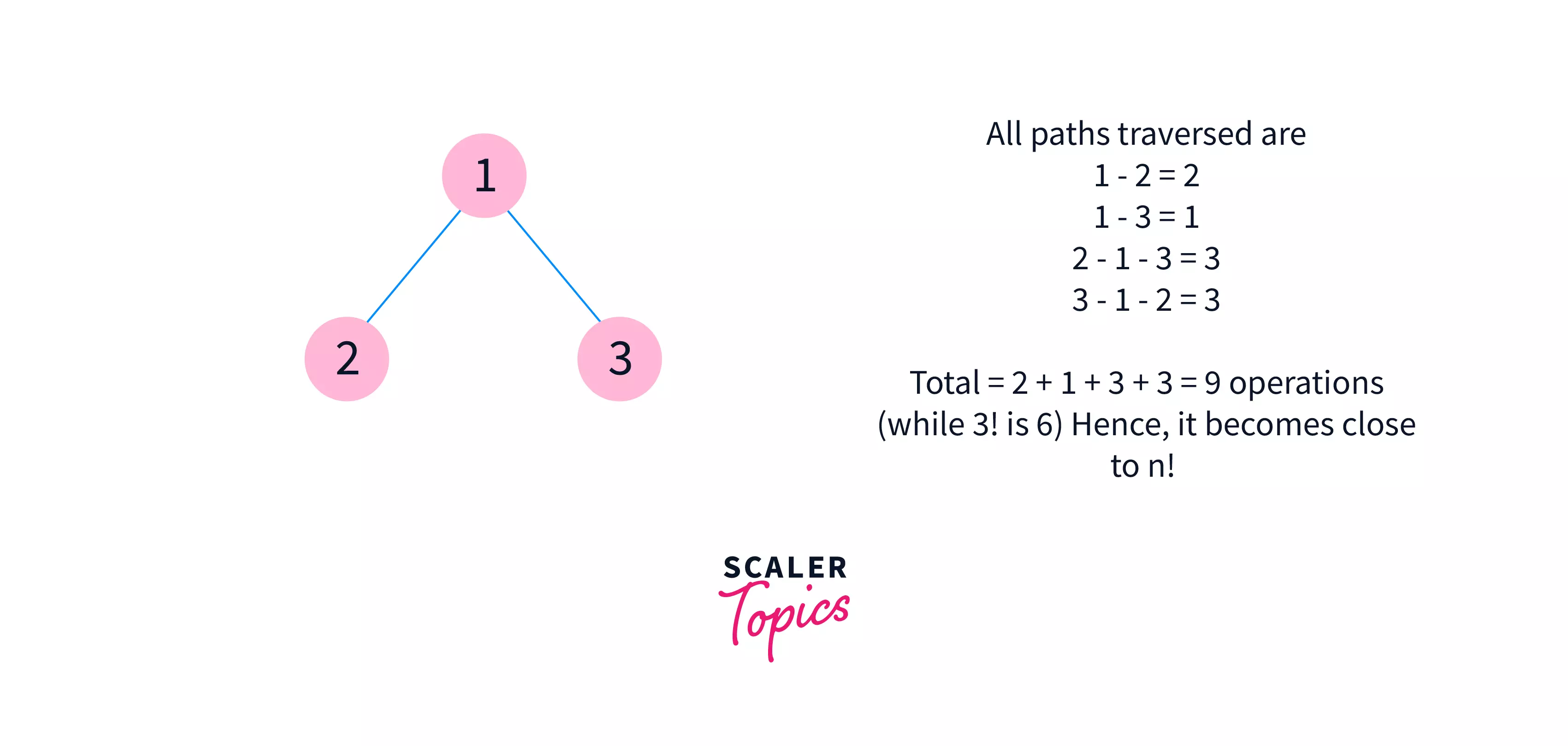
Time Complexity: It can be seen that we are performing a depth-first search from each of the n vertices and in the worst case it may take time complexity close to O(n!).Let's understand it with the exampler image below:

Let's look at yet another and more efficient approach of checking a Hamiltonian path in a graph.

3) Dynamic Programming Approach

In this approach as the name suggests we need to store the memos (memo can be interpreted as memory) of the small solutions to build larger solutions, but the question is what are those small problems and their solutions to store and how to build a memo based solution for the Hamiltonian Path, we will answer all these questions in the following section

Consider again the same problem of Ray visiting the houses of his friends in his neighborhood, in the naive approach we simply had to generate all paths and check for each of them whether it is a Hamiltonian Path or not but in this solution we are doing a lot of redundant work like for example refer to the image below:

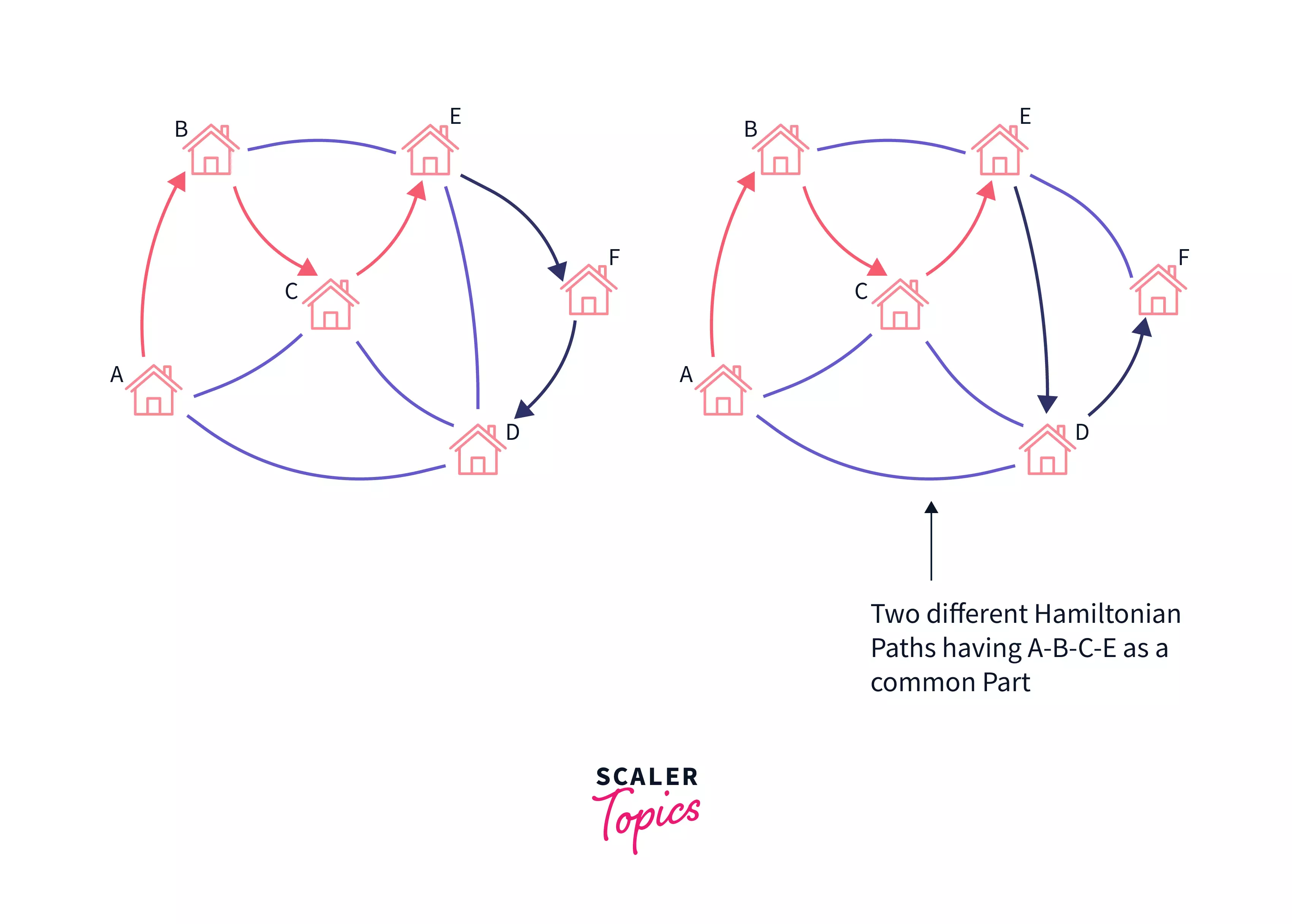
In the figure above, the two Hamiltonian Paths {A, B, C, E, F, D} and {A, B, C, E, D, F} are separately generated by the previous approach, but we can observe that the part {A, B, C, E} (Marked with red edges) is common to both Paths which is redundant work. This can be stored in a memo and quickly used while building the paths that visit the next unvisited nodes like {A, B, C, E, D} and {A, B, C, E, F}. In these paths, we simply added edges E-D and E-F to the previously memoized path {A, B, C, E}, which can be quickly retained because we stored it previously, and these new paths can also be memoized in the same way we did for {A, B, C, E}. And so on, until we visit all the vertices of the graph exactly once, and once this happens, we are already done with the problem.

Now, using the above idea of storing partial paths and building the solution towards final Hamiltonian Paths, we shall be emphasizing the questions like implementing the above strategy in practice in the best possible way and the working solution of the problem, so let's jump to the implementation part.

Implementation of Dynamic Programming Approach: We have learned about partial solutions or partial paths in this specific case, we can conclude that those partial paths are simply the subsets of the vertices of the graph where there is a path in the subset that visits every single vertex in it and ends at some vertex, in other words, we build larger subsets(Hamiltonian paths) from the smaller subsets(Hamiltonian paths)
Let's understand the idea with the following example:

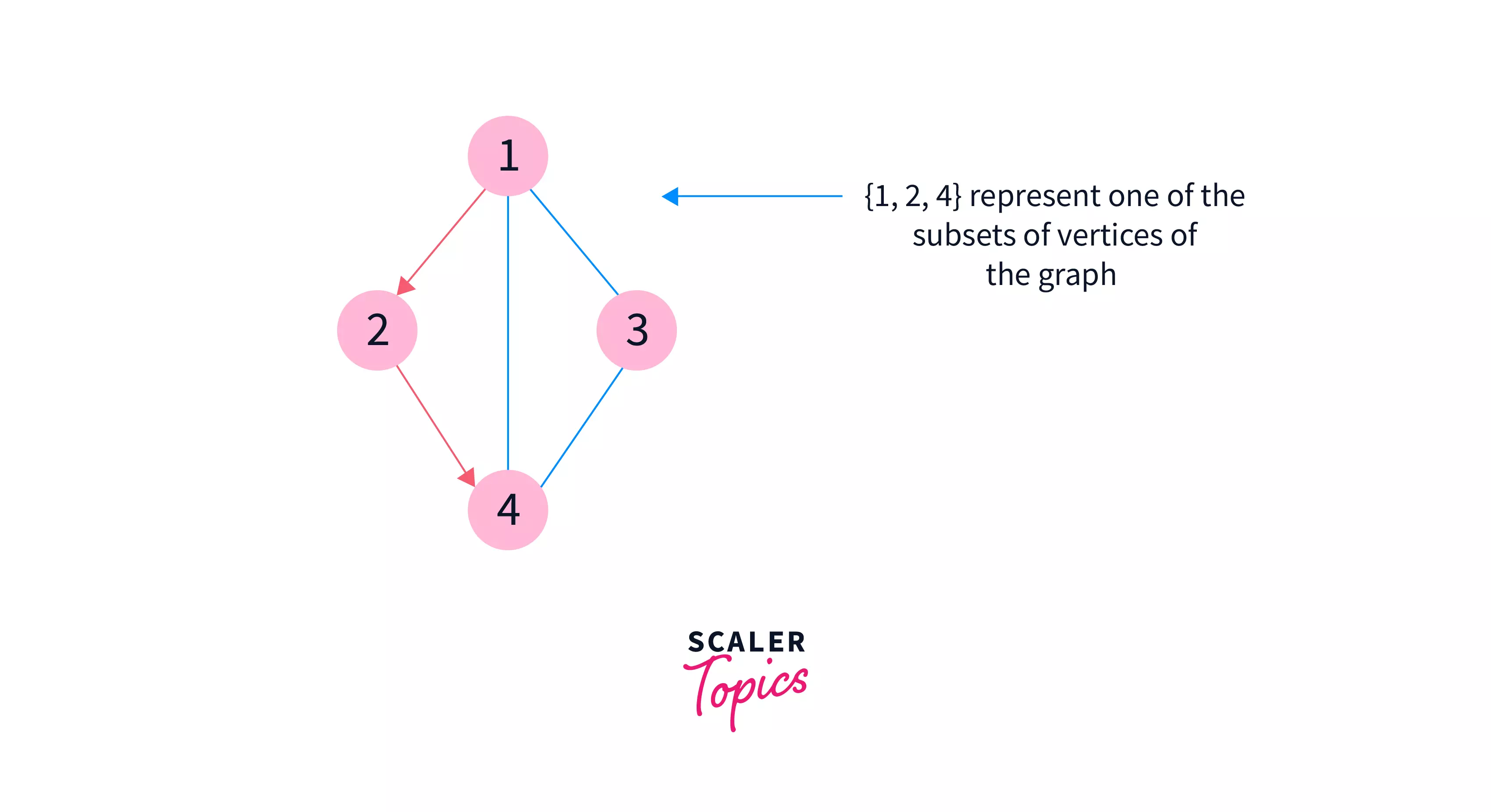
In this graph, U = {1,2,4} is one of the 16 subsets of the vertices of the graph. In this subset we observe that there exists a path that visits all vertices and ends at 4. Now, let's consider another subset i.e. V = {1,2} and ask ourselves does there exist a path that visits every vertex in V exactly once and ends at 2, the answer is yes there exists such path. Now let's get back to the previous subset U which is just V + 4 (here + represents the addition of vertex in the subset).

We know at this point that V is a subset where there is a path that visits each and every vertex exactly once and it ends at 2, simply extending this vertex 2 to add 4 to make the subset U. Now, U is a subset which contains a path that visits every vertex exactly once and ends at 4.

Hence, we built the larger subset U with a valid path from a smaller subset V with a valid path and in the implementation, we start processing from smaller subsets and build larger ones. The next question is that how to represent those subsets, one of the ways is to use bitmasking. Let's understand the Pseudocode implementation:

In the above implementation, graph[][],n represents the given graph represented in the adjacency matrix form and the number of vertices in the graph. $dp[n][2^n]$ is a boolean matrix is used to check for the existence of hamiltonian paths in different subsets which are represented by bitmasks while there are total $2^n$ subsets including the empty subset(because in bitmask of size n, there are two ways either to select a vertex or not), dp[j][i] represents the existence of the path in mask(subset) i that ends at j.

Introduction to Euler's Path

• Degree of a vertex is the number of incident edges on it.
• Euler's path unlike Hamiltonian Path visits each edge.
• Degree of vertices helps to determine the existence of Euler's path in a graph.

Let's take the same example of Ray visiting his friends on this Christmas. Ray decides to distribute gift cards that he prepared this year to preach the gospel and he wants to distribute it to as many people as he can. Therefore, he decides to visit all streets in his neighborhood and his task is to find such path which visits every single street of the given network of houses exactly once and one of such paths is as shown below:

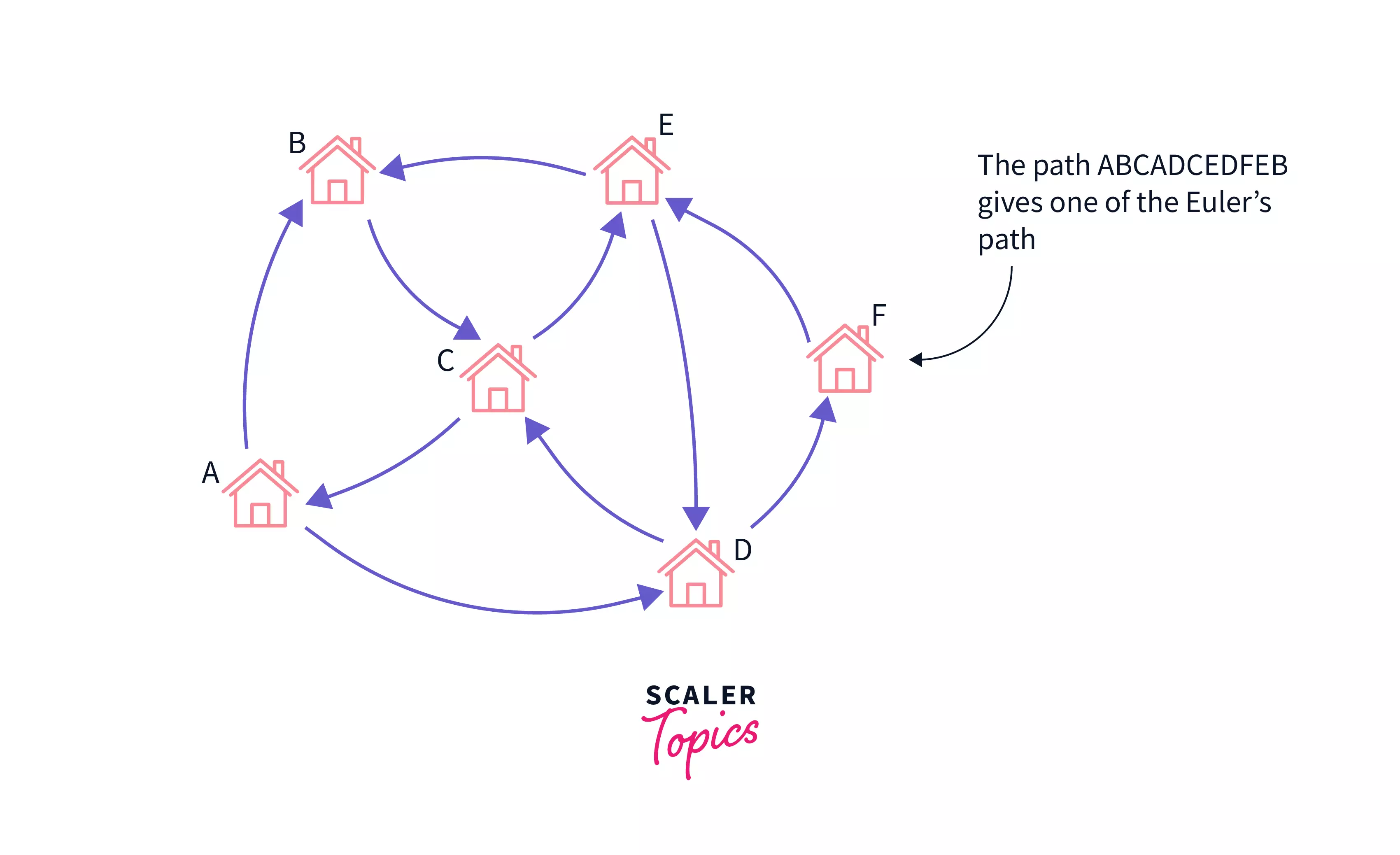
The path ABCADCEDFEB visits every single street of the network of houses and it is obvious that there may exist more than one such path (Try enumerating all of them) in such graph and in computer science, they call it Euler's path and it may exist in directed as well as undirected networks the example of Ray visiting neighbors is a case of the undirected network where each street is a two-way street. Let's jump into the formal definition of Euler's path.

Definition of Euler's Path

• Euler's path in a finite connected graph is a path that visits every single edge of the graph exactly once Although it allows the revisiting of the vertices. It is also called Euler's trail or Eulerian's trail
• It exists in directed as well as undirected graphs and for the Eulerian path to exist in these graphs there are certain theorems and lemmas for directed as well as undirected graphs and some of them are explained below.
• The graph component must be connected for the Euler's path to exist in that particular component and all vertices with non-zero degrees must belong to the same connected component.

Now, once we know the definition of the Euler's path, the next question is how to make sure or identify for a given connected graph that there must exist an Eulerian Trail or not without tracing every single path. Let's look at theorms to identify such paths in connected graphs.

Euler's Theorem for Euler's Path

This theorem is used to check whether a connected graph contains an Euler's path or not, before jumping to the definition let's understand a few terms.

1) Degree of a Vertex: In a graph, the degree of a vertex is defined as the number of edges incident to it.

2) Euler's circuit: In a connected graph, It is defined as a path that visits every edge exactly once and ends at the same vertex at which it started, or in other words, if the starting and ending vertices of an Euler's Path are the same then it is called an Euler's circuit, we will be discussing this in detail in the next section.

Refer to the image below to have a better understanding of the degree.

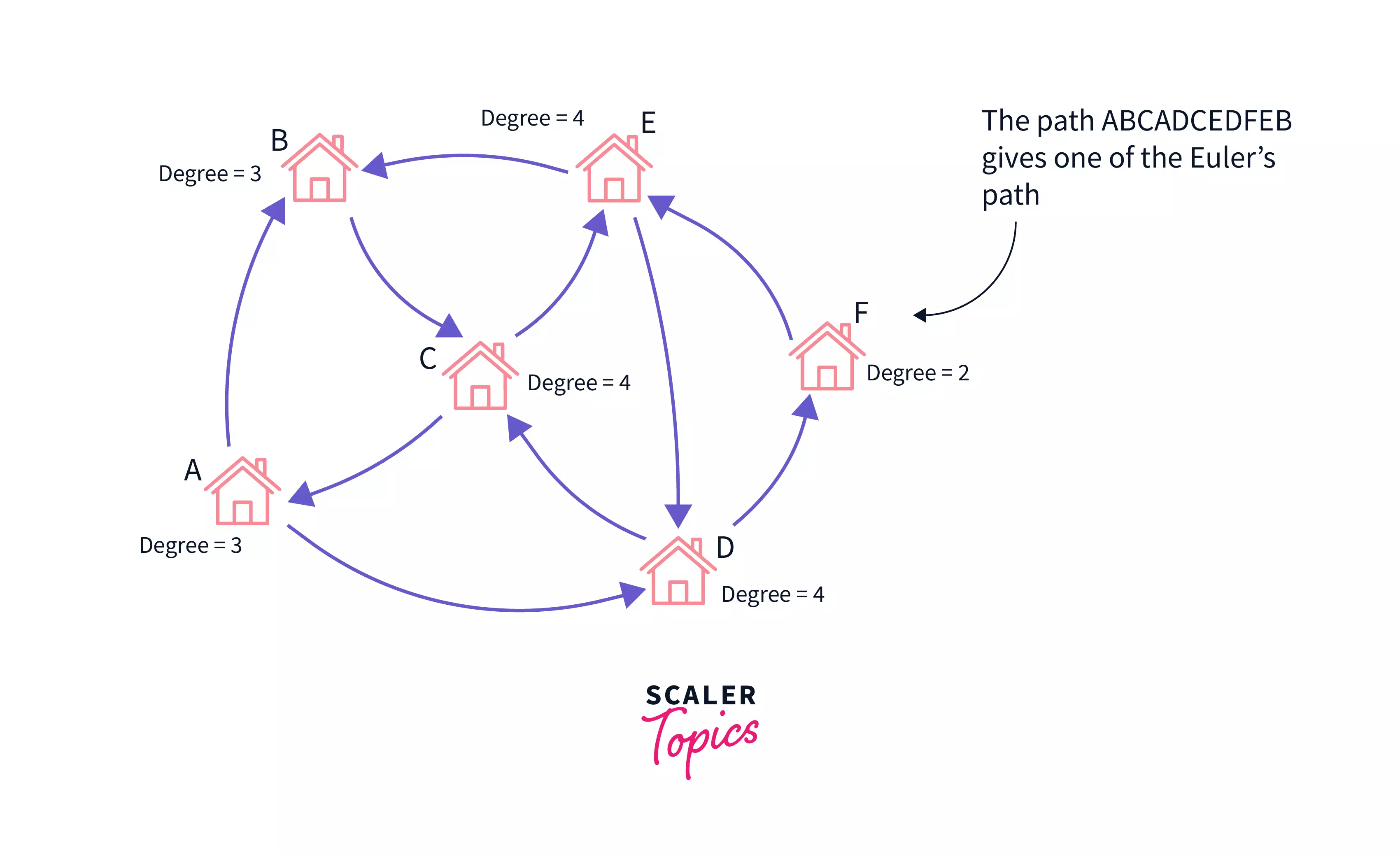
The theorem states that if a graph has exactly two odd degree vertices, then it has exactly one Euler Path, but no Euler Circuit, Also the Euler Path must start at one of the odd vertices and end at another.

It can be seen in the example of Ray visiting his neighborhood, the network has exactly two vertices of odd degree i.e. vertex A and B which are indeed starting and ending vertices of the Euler's Path.

After we learned about Euler's Path, there is another interesting and close concept in the same context that is called Euler's Circuit Let's discuss that in the next section.

Introduction to Euler's Circuit

• Degree of a vertex is the number of incident edges on it.
• Euler's circuit is also a Euler's path with same ending and starting vertex.
• Degree of vertices helps to determine the existence of Euler's Circuit in a graph.

In the context of Euler's Path, there is another concept called Euler's Circuit which is quite useful while solving some of the graph problems, Let's take a new example for understanding the same, then we will come back to the conclusion why the same example of Ray cannot be used here.

Imagine the graph shown below, In this case Ray starts at the house A and ends at the same after visiting all edges exactly once although he is visiting same house more than once.

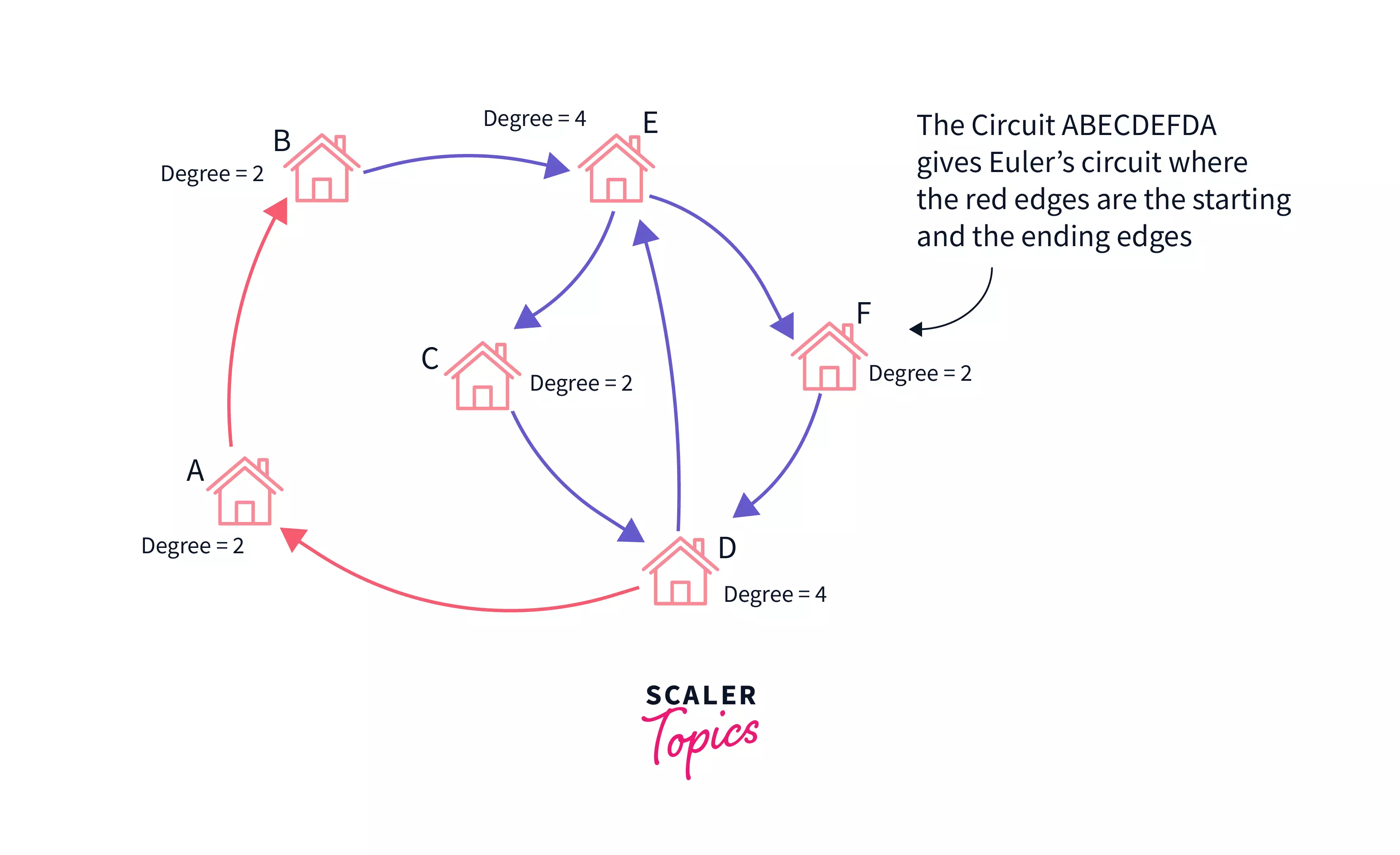
Here, the path ABECDEFDA visits every edge exactly once and starts and ends at the same vertex, this path is called Euler's Circuit because it is a closed path.

Let's jump to the formal definition of the same

Definition of Euler's Circuit

• Euler's Circuit in finite connected graph is a path that visits every single edge of the graph exactly once and ends at the same vertex where it started. Although it allows revisiting of same nodes. It is also called Eulerian Circuit.
• It exists in directed as well as undirected graphs. For the Eulerian Circuit to exist in these graphs there are certain theorems and lemmas for directed as well as undirected graphs and some of them are explained below.
• The graph component must be connected for the Euler's Circuit to exist in that particular component and all vertices with non-zero degrees must belong to same connected component.

Now, once we know the definition of the Euler's Circuit, the next question is how to make sure or identify for a given connected graph that there exist an Eulerian Circuit or not without tracing every single circuit. Let's look at theorems to identify such paths in connected graphs.

Euler's Theorem for Euler's Circuit

This theorem is used to check whether a connected graph component contains an Euler's path or not.

It states that if all the vertices of a graph component have an even degree (Excluding 0), then it must have an Euler's Circuit in it and Euler's Circuit can start and end at any vertex.

It is explicit in the image given above in the example each vertex has even degree and it is obvious that there can be more than one Euler's circuit in it for example DABECDEFD is also an Euler's Circuit (try enumerating all of them).