Interpolation Search

This is the third part of a three-part series on Searching Algorithms.

In the previous article about binary Search, we discussed one of the best searching algorithms out there.

If you didn’t get a chance to read that one, hop right over to it and have a quick read.

Today, we’ll be discussing an improvement over the traditional Binary Search approach called Interpolation Search. Yes, you heard it right; we can still do a little better than Binary Search.

Definition

As you probably know by now; Binary search works great if the data set is sorted. But can we do better? Let’s see when and how.

Interpolation Search

In a typical English dictionary, data is quite uniformly distributed, For example, all the words starting with a or b will be in the beginning of the dictionary, and all the words starting with y and z will be in the very end of the dictionary. On the other hand, words starting with m and n will probably lie somewhere in the middle.

angle, binary, …………………., yesterday, zoo

Names in a typical English dictionary sorted in increasing order

So if we want to search a word like binary, the natural human instinct will be to start the search in the beginning of the dictionary because we know that’s where all the words starting with b must lie.

On the other hand, if we want to search for a word like zoo, you might start in the search in the latter half of the dictionary.

To simplify, it doesn’t always make sense to always start in the middle of the data set. Rather, we can start our search at a different position each time, based on the element we need to search. Since the data is uniformly distributed, the probability of finding the element near a specific position will be higher.

The above example is the principle on which Interpolation Search is primarily based; the human instinct to find an element in a uniformly distributed sorted data set.

How Does Interpolation Search Work?

Unlike Binary Search which always starts the search from the middle of the array, Interpolation Search tries to find the element where it is more likely present.

In a uniformly distributed array, larger numbers will lie towards the end of the array whereas smaller ones will lie in the beginning. So, Interpolation Search tries exactly that.

For larger numbers, it’ll start the search somewhere in the end of the array and for smaller numbers, somewhere in the beginning.

So how can we define if data is uniformly distributed or not? Let’s see with some examples.

As you can see above, the values in the above array range from 1 to 500000 while there are only 8 values in the array. The values are increasing almost exponentially here. Hence, the values are not uniformly distributed in the above array.

In the above array, the values range from 2 to 18, and there are a total of 8 elements. The values are increasing in a linear manner here. Hence, the above array is much more uniformly distributed than before.

Another easier way to check uniformity is that we can check the difference between subsequent elements of the data set. If the difference is almost consistent and not changing significantly, i.e. the delta is similar for all the elements, then we can say the data set is uniformly distributed.

Now that we know what a uniformly distributed data set looks like, how do we decide the position where we need to start the search from? Head’s up, a cool mathematics equation solution ahead 🙂

If you recall some high school mathematics, the equation for a straight line is

$y = m*x + c$

where

x: coordinate along the horizontal axis
y: coordinate along the vertical axis
m: the slope of the line
c: a constant

If the array is uniformly distributed, we can say that it will follow the path of a straight line and hence,we can represent the elements of the array using the above equation as follows.

$arr[index] = m*index + c$

where

index: the position of the element in the array
arr[index]: the value at this index in the array

Let’s replace the above equation with low and high which represents the lowest and the highest index of the array at any point in time.

$arr[low] = m*low + c$ —– (1)

$arr[high] = m*high + c$ —– (2)

Now let’s say we are trying to search for an element, K in this array. Then replacing K in the above equation, we get

$K = m*index + c$ —– (3)

where index is the probable position of K in this array.

If we subtract equation (1) from (2), we get

arr[high] – arr[low] = m * (high – low)

m = (arr[high] – arr[low]) / (high – low) —– (4)

Now if we subtract equation (1) from (3), we get

K – arr[low] = m * (index – low)

index – low = (K – arr[low]) / m

index = low + (K – arr[low]) / m

Replacing the value of m from equation (4) above, we get

$index = low + (K-arr[low])*(high-low)/(arr[high]-arr[low])$

So there we have it, the magic equation which we can use to calculate the index at which we should start the search process for any element K.

So rather than always starting at the middle of the array-like Binary Search, we use the above equation to calculate the index at which we will start the search process.

Once we calculate this index, the rest of the process is the same as Binary Search. We compare the element at the particular index calculated above with K.

If the value is less than K, we ignore the left half of the array and calculate the next index where we start our search for the right half of the array.

On the other hand, if the value is more than K, we ignore the right half of the array and calculate the next index where we start our search for the left half of the array.

If the value at the index is equal to K, we have found the element K in the array and our job is done.

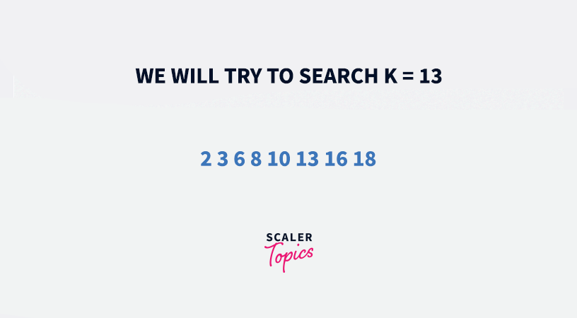
Let’s try to apply this approach to the given array.

We will try to search K = 13 in the above array. The size of the array is 8.

low = 0, high = 7, arr[low] = 2, arr[high] = 18

Replacing the above values in the above equation to find index, we get

If the value of index is a decimal, we round off the value to its nearest integer or its floor value.

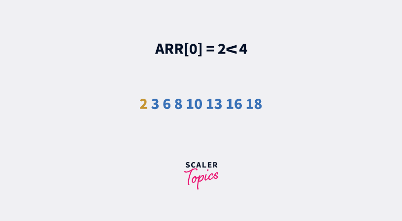
So rather than starting at the middle, we start our search at the index = 4 of the array.

Since the element at index = 4 is less than K = 13, we ignore the left half and try again in the right half.

2 3 6 8 10 13 16 18 ignore left half

low = 5, high = 7, arr[low] = 13, arr[high] = 18

index = 5 + (13 – 13) * (7 – 5) / (18 – 13) = 5

2 3 6 8 10 13 16 18 arr[5] = 13 == 13, found K

And there we have it, we found the element K = 13 in the second comparison.

Let’s try to find an element that is not present in the array, K = 4.

In this case, we start the search at the index = 0 of the array.

index = 0 + (4 – 2) * (7 – 0) / (18 – 2) = 0.875 ~ 0

$2 3 6 8 10 13 16 18 arr[0] = 2 < 4$

So, we ignore the left half of the array, and apply the same process for the right half of the array.

2 3 6 8 10 13 16 18 ignore left half

**low = 1, high = 7, arr[low] = 3, arr[high] = 18 **

**index = 1 + (4 – 3) * (7 – 1) / (18 – 3) = 1.4 ~ 1 **

$2 3 6 8 10 13 16 18 arr[1] = 3 < 4$

Again, we ignore the left half of the array and apply the same process for the right half of the array.

2 3 6 8 10 13 16 18 ignore left half

**low = 2, high = 7, arr[low] = 6, arr[high] = 18 **

**index = 2 + (4 – 6) * (7 – 2) / (18 – 6) = 1.16666 ~ 1 **

2 3 6 8 10 13 16 18 arr[low] = 6 > 4

Since the value of K is less than arr[low] and the array is sorted, it means the element K cannot be present in the subarray between [low, high], which is quite evident since 4 is not present in the array.

2 3 6 8 10 13 16 18 ignore right half

As you can see, we were able to determine whether an element was present in the array or not much quicker than we did with Binary Search, if and only if the array is sorted and uniformly distributed.

Algorithm

Below is the algorithm of Interpolation Search.

1. Initialise n = size of array, low = 0, high = n-1. We will use low and high to determine the left and right end of the array in which we will be searching at any given time.
2. if low > high, it means we have exhausted the array and we could not find K. We return -1 to signify that the element K was not found
3. if K < arr[low] || K > arr[high], it means K is either less than the smallest element or greater than the largest element of the current array and since the array is sorted, we will never be able to find K in this array. Hence, we return -1 to signify that the element K was not found
4. else low <= high, and we apply the interpolation equation to find the index where we should start the search from , as follows:
   • Initialise index = low + (K-arr[low])*(high-low)/(arr[high]-arr[low])
   • if arr[index] < K, it means the element at the current index is less than K. Thus, all the elements in the left side of the index will also be less than K. Hence, we repeat step 2 for the right side of the index. We do this by setting the value of low = mid+1, which means we are ignoring all the elements from low to index and shifting the left end of the array to index+1
   • if arr[index] > K, it means the element at the current index is greater than K. Thus, all the elements in the right side of the index will also be greater than K. Hence, we repeat step 2 for the left side of the index. We do this by setting the value of high = index-1, which means we are ignoring all the elements from index to high and shifting the right end of the array to index-1.
   • else arr[index] == K, which means the element at the current index is equal to K and we have found the element K. Hence, we do not need to search anymore. We return the value of index directly from here signifying that index is the position at which K was found in the array.

Implementation

Below is an implementation of Interpolation Search in Java 8.

Output:

Time Complexity

If the data set is sorted and uniformly distributed, the average case time complexity of Interpolation Search is O($log_2(log_2(N)$) where N is the total number of elements in the array.

On the other hand, if the data is sorted but quite randomized, the time complexity of Interpolation Search will be much worse than Binary Search. In fact, it’ll be almost similar to Linear Search, i.e. O(N). Ouch!

Space Complexity

It’s quite evident that we are not using any significant extra memory in Interpolation Search. So the space complexity is constant, i.e. O(1).

P.S. The variables used for storing the bounds, index and other minor information are constant since they don’t depend on the input size of the array.

Applications

Since the major requirement to use Interpolation Search is that the data set must be sorted and uniformly distributed, it has a very limited number of applications in real life, where data is actually quite randomised.

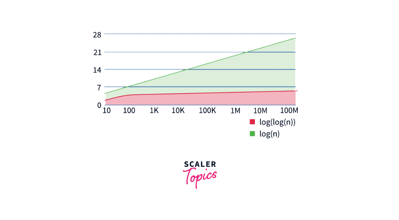
Nevertheless, if the data is indeed uniformly distributed, Interpolation Search performs a lot better than Binary Search as it’s evident from the below image.

Ignite Data Structures Brilliance! Enroll in Scaler Academy's Online DSA Course to Hone Your Coding Skills.