Johnson’s Algorithm

Overview
Johnson’s Algorithm is used to find all pair shortest path in a graph. We can use the Johnson's Algorithm to find the shortest paths between all pairs of vertices in an edge-weighted directed graph. Johnson's Algorithm uses both Dijkstra's Algorithm and Bellman-Ford Algorithm.
Johnson’s Algorithm can find the all pair shortest path even in the case of the negatively weighted graphs. Although we can use the Floyd Warshall's Algorithm in order to find the all pair shortest path in the graph though Johnson’s Algorithm is much more efficient in terms of time complexity than the Floyd Warshall's Algorithm.
Takeaways
- Complexity of Johnson’s Algorithm
- Time complexity -
Introduction to Johnson’s Algorithm
Consider a situation where a Road Construction firm has been given a tender to connect multiple villages via road network in such a way that the people can reach from one village to another in minimum possible time.
We can represent the road network as a graph where the villages can be represented in form of the nodes of the graph and the road between the villages can be represented in form of edges of the graph.
Now this problem is reduced to finding the minimum distance between all pairs of nodes in a graph.
Johnson’s Algorithm is used to find all pair shortest path in the given graph G. This problem of finding the all pair shortest path can also be solved using Floyd warshall Algorithm but the Time complexity of the Floyd warshall algorithm is , which is a polynomial-time algorithm, on the other hand, the Time complexity of Johnson’s Algorithm is which is much more efficient than the Floyd warshall Algorithm. So we can say that Johnson’s Algorithm is an Optimised Approach to find all pair shortest path in a graph.
Johnson's Algorithm uses both Dijkstra's Algorithm and Bellman-Ford Algorithm. Johnson's Algorithm can find the all pair shortest path even in the case of the negatively weighted graphs. It uses the Bellman-Ford algorithm in order to eliminate negative edges by using the technique of reweighting the given graph and detecting the negative cycles.
Now once we come up with this new, modified graph, then this algorithm uses Dijkstra's shortest path algorithm to calculate the shortest path between all pairs of vertices for a given graph.
The output of Johnson’s algorithm is the set of shortest paths between every pair of vertices in the original graph. The above steps are discussed in detail below.
Transform Your Career
Choose from our industry-leading programs designed for career success
Modern Software and AI Engineering Program
Master full-stack development with AI integration

Modern Data Science and ML with specialisation in AI
Advanced data science techniques with AI specialization
Advanced AIML with Specialisation in Agentic AI
Deep dive into AIML with focus on Agentic systems
DevOps, Cloud & AI Platform Engineering
Build and manage AI-powered cloud infrastructure
AI Engineering Advanced Certification by IIT-Roorkee
Premier AI engineering certification from IIT-Roorkee
Three Main Parts of Johnson's Algorithm
The working of Johnson's Algorithm can be easily understood by dividing the algorithm into three major parts which are as follows
- Adding a base vertex
- Reweighting the edges
- Finding all-pairs shortest path
Now we will learn about each of the three main parts of Johnson's Algorithm in great detail. Let us understand the working of Jhonson's Algorithm with an example.
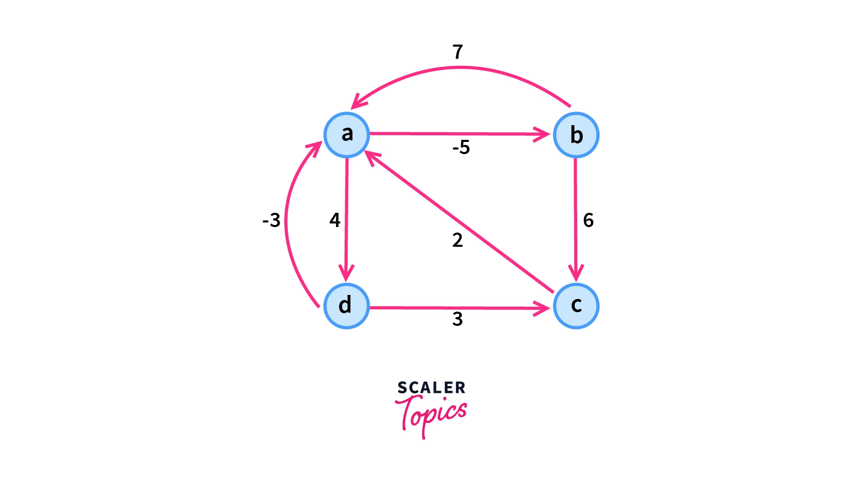
Consider an edge-weighted directed graph having four vertices which are ,, and as shown in the picture below. Our goal is to calculate the shortest path between every pair of vertices in the given graph .
Adding a Base Vertex
To calculate the shortest path between every pair of vertices the idea is to add a base vertex (vertex in figure below) that is directly connected to every vertex. In other words, the cost to reach each vertex from the newly added base vertex is zero. Since at this stage our graph contains negative weight edges so we apply the Bellman-Ford Algorithm.
Let the modified graph with the newly added base vertex be ' which is shown in the image below. Now after applying the Bellman-Ford Algorithm for the above-modified graph ' , we get the shortest distance from the base vertex to all other vertices which is as follows.
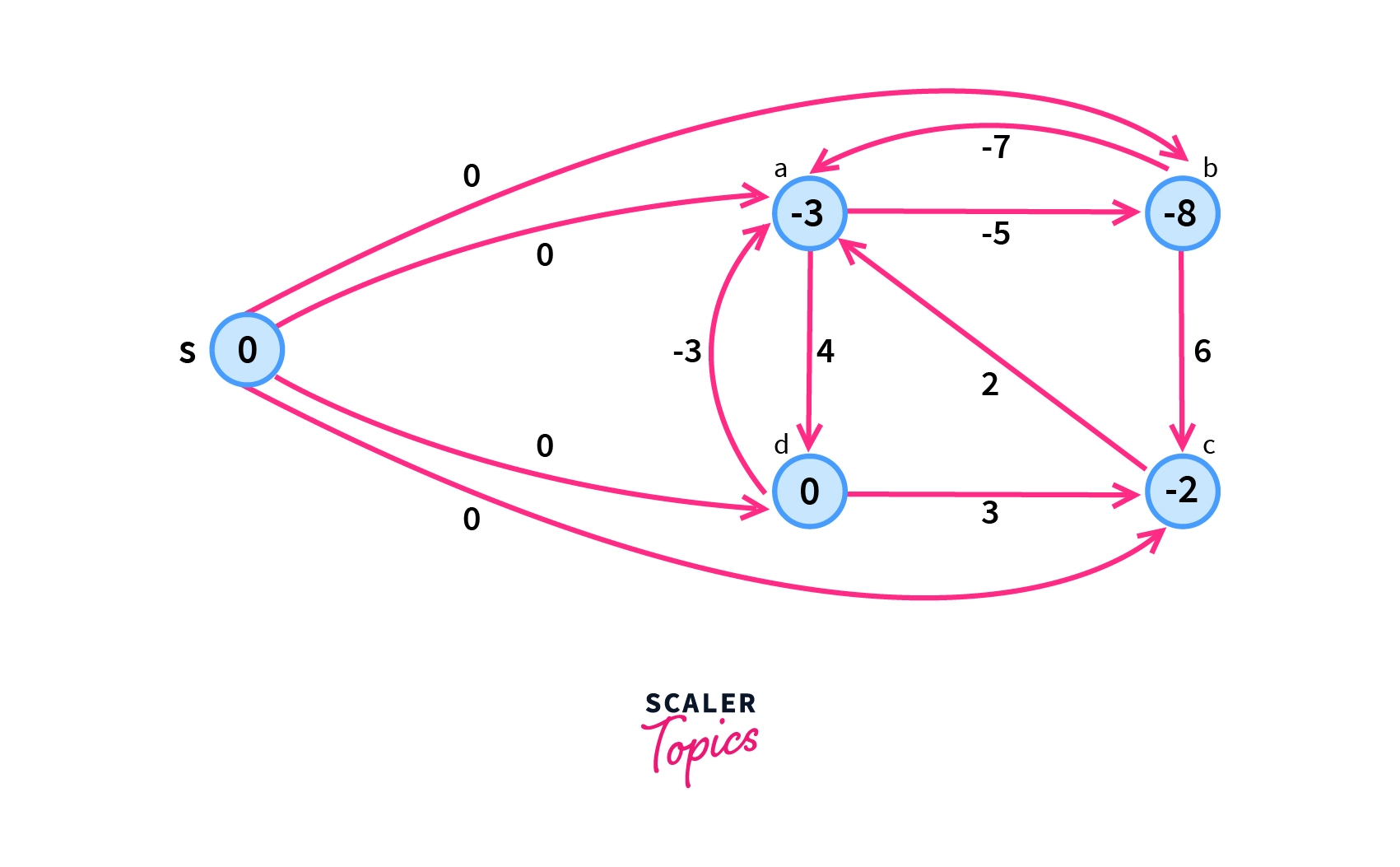
where D(S,V) is the shortest distance from the vertex S to the vertex V.
Reweighting the Edges
Johnson's Algorithm uses the technique of reweighting of the edges.
Reweighting is a process by which edge weight is changed to satisfy following two properties.
- For all pairs of vertices u, v in the graph, if a certain path is the shortest path between those vertices before reweighting, it must also be the shortest path between those vertices after reweighting.
- For all edges, (u, v), in the graph, weight(u, v) must be non-negative.
Reweighting of the edges is done because of the fact that if the weight of all the edges in a given graph G are non negative, we can find the shortest paths between all pairs of vertices just by running Dijkstra's Algorithm once from each vertex which is more efficient than applying the Bellman-Ford algorithm.
Now, the new set of edges weight W which is obtained by reweighting the edges must satisfy the following essential properties.
- For all pair of vertices u, v ∈ V, the shortest path from u to v using weight function W is also the shortest path from u to v using weight function W.
- For all edges (u, v), the new weight W (u, v) is non negative.
Now as we already got these distances of all the vertices from the base vertex S, we remove the source vertex S and reweight the edges using the following formula.
By using the triangle inequality, we have
So, by using the above equation we can define our reweighting equation as follows.
where W(u,v) is the original weight of an edge between the vertices u,v and D(S,V) is the shortest distance from the vertex S to the vertex V.
Now we calculate the new weights by using the above formula.
For the edge a to b, putting u=a amd v=b in the above formula, we get
For the edge b to c, putting u=b amd v=c in the above formula, we get
For the edge d to c, putting u=d amd v=c in the above formula, we get
For the edge a to d, putting u=a amd v=d in the above formula, we get
For the edge c to a, putting u=c amd v=a in the above formula, we get
For the edge b to a, putting u=b amd v=a in the above formula, we get
For the edge d to a, putting u=d amd v=a in the above formula, we get
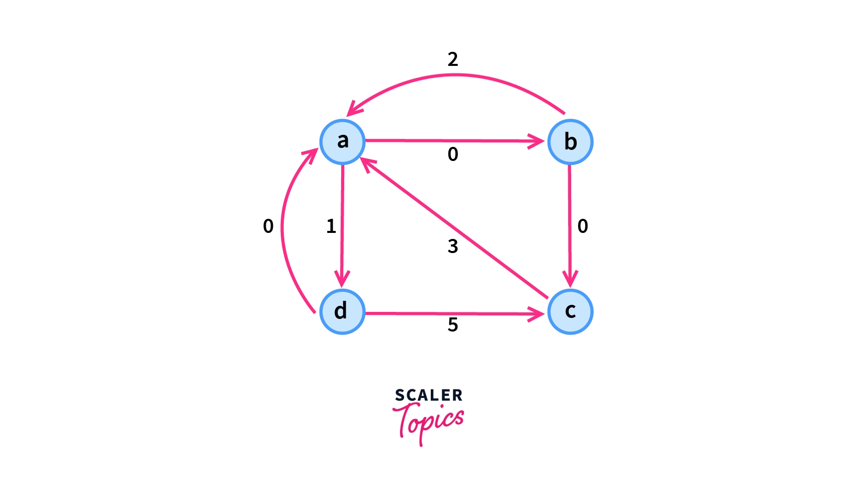
The Picture below shows the graph with the reweighted edges.
Finding the All-pairs Shortest Path
Now after we have reweighted the weight of the edges, we have got all the edges with the non-negative weights so we can apply the Dijkstra's Algorithm to find all pair shortest path for a given graph .
After getting the shortest path for each pair of vertices it becomes very important to transform these path weights back into the original path weights so that an accurate path weight is returned at the end of the algorithm. This can be done by simply reversing the reweighting process. Finally, we get the matrix that represents the shortest path from each pair of vertices.
Now, after applying Dijkstra's Algorithm on each vertex individually, we get the shortest distance between all pairs, which is as follows.
Consider a as source vertex, the shortest distance from a to all other vertices are as follows.
Consider b as source vertex, the shortest distance from b to all other vertices are as follows.
Consider c as source vertex, the shortest distance from c to all other vertices are as follows.
Consider d as source vertex, the shortest distance from d to all other vertices are as follows.
From the above calculation, we can represent the shortest distance between all pairs shortest paths in form of a table. The table below represents the distance between every pair of vertices.
Please note that in case of directed edge-weighted graph the distance from any vertex u to vertex v and vice versa may or may not be same like distance from vertex a to vertex b is 0 unit but distance between vertex b to vertex a is units.
| Distance | a | b | c | d |
|---|---|---|---|---|
| a | 0 | 0 | 0 | 1 |
| b | 2 | 0 | 0 | 3 |
| c | 3 | 3 | 0 | 4 |
| d | 0 | 0 | 0 | 0 |
Turn Learning into Career Growth
Reweighting Proof
Now we have reweighted the edges of the graph. So we need to prove that reweighting the graph does not actually change the overall sum of weights of the edges. In the reweighted graph, we add the same quantity − where and are the length of the shortest path from the newly added base vertex S to the vertex s and vertex respectively. in all paths between a pair s and t of nodes added to them.
Let us see how we can mathematically prove that the concept of reweighting preserves the actual overall sum of weights of the edges. Let be a path between two vertices of the graph say . Its weight in the reweighted graph is given by the following expression:
The expression below is the weight of p in the original weighting.
(w(s,p1)+h(s)-h(p1))+(w(p1,p2)+h(p1)-h(p2))+...+(w(pn,t)+h(pn)-h(t))
Every +h(pi) is cancelled by -
h(pi) in the previous bracketed expression therefore, we are left with the following expression for W:
(w(s,p1)+w(p1,p2)+...+w(pn,t))+h(s)-h(t)
So we can clearly see that the reweighting adds the same amount to the weight of every path from vertex to vertex t, so we can say that a path is the shortest path in the original graph if and only if it remains the shortest path after reweighting of the graph.
Now once there is no existence of negative edges, we are sure to have the optimality of the paths which are found by Dijkstra's algorithm. The distances in the original graph may be calculated from the distances calculated by Dijkstra's algorithm in the reweighted graph by reversing the reweighting transformation.
Algorithm Pseudocode
- Firstly we will create a modified graph G' in which we will add the base vertex to the original graph G.
- We will apply the Bellman-Ford ALgorithm to check whether the graph G' contains the negative weight cycle or not.
- We can find all pair shortest path only if the graph is free from the negative weight cycle.
- Once we found that the graph is free from the negative weight cycle then we calculate the shortest path for each vertex using Bellman-Ford algorithm.
- We also reweight the edges of the graph by removing the base vertex which will also assure us that the graph will be free from any negative-weight edges.
- Now at this stage since we have reweighted the edges our graph is guaranteed to be free from negative-weight edges so we apply the Dijkstra Algorithm for each vertex in the graph in order to find the shortest distance between every pair of vertex in the graph which is our desired goal.
Below is the Pseudocode for Johnson’s Algorithm.
Implementation of Johnson's Algorithm
- Firstly we will create a list to store the modified wights which are represented by Altered_weights in the code below.
- We will apply the Bellman-Ford algorithm to find the modified weights.
- Our modified graph which is represented by Altered_Graph in the code below would consist of Altered_weights and it will be free from negative-weight edges.
- Now at this stage since our Altered_Graph is guaranteed to be free from negative-weight edges, we apply the Dijkstra Algorithm for each vertex in the Altered_Graph in order to find the shortest distance between every pair of vertex in the graph which is our desired goal.
Below is the implementation of Johnson’s Algorithm in Python.
Output of Above Program
Time Complexity of Johnson’s Algorithm
Since the main steps required in Johnson's Algorithm are:
- Bellman-Ford Algorithm which is called once.
- Dijkstra Algorithm which is called V times, where V is the number of vertices in the given graph G.
We know that the Time complexity of:
So overall time complexity is which is average case.
It is really interesting to know that in case of the complete graph the time complexity of Johnson's algorithm becomes the same as that of the Floyd Warshell Algorithm.
It is important to note that the Worst-case Time complexity of the Jhonson's algorithm is as Dijkstra's Algorithm takes time.
Applications of Johnson's Algorithm
There are various applications of Jhonson's Algorithm some of them are as follows.
- The most widely used application of the Johnsons Algorithm is the Networking of Roads.
- Used for Network Routing for choosing the optimal path for sending the data packets.
- Also used in Driving Directions for telling the best route with the shortest path and least traffic congestion.
- This algorthim is widely used for Logistics purpose by different firms to minimise their transportation cost.
Conclusion
- In this article, we have learned about Johnson's Algorithm.
- We have also learned about the working of Johnson's Algorithm.
- We compared Johnson's Algorithm with the Floyd Warshall Algorithm.
- We saw how Johnson's Algorithm uses Dijkstra's Algorithm and Bellman Ford's Algorithm to increase the efficiency of the Johnson's Algorithm over the Floyd Warshall Algorithm in terms of time complexity.
- We have learned how to implement Johnson's algorithm.
- We also analyzed the time complexity of this algorithm.
- We saw some interesting real-life applications of this algorithm.