Load Factor and Rehashing

Complexity and Load Factor

1. The time taken in the initial step is contingent upon both the value of K and the chosen hash function. For instance, if the key is represented by the string "abcd," the hash function employed might be influenced by the length of the string. However, as n becomes significantly large, where n is the number of entries in the map, and the length of keys becomes negligible compared to n, the hash computation can be considered to occur in constant time, denoted as O(1).

2. Moving on to the second step, it involves traversing the list of key-value pairs located at a specific index. In the worst-case scenario, all n entries might be assigned to the same index, resulting in a time complexity of O(n). Nevertheless, extensive research has been conducted to design hash functions that uniformly distribute keys in the array, mitigating the likelihood of this scenario.

3. On average, with n entries and an array size denoted by b, there would be an average of n/b entries assigned to each index. This n/b ratio is referred to as the load factor, representing the burden placed on our map.

4. It is crucial to maintain a low load factor to ensure that the number of entries at a given index remains minimal, thereby keeping the time complexity nearly constant at O(1).

• Complexity of Hashing

  • Time complexity - O($n$)
  • Space complexity - O($n$)

• Complexity of Rehashing

  • Time complexity - O($n$)
  • Space complexity - O($n$)

Load Factor Example

Let’s understand the load factor through an example.

If we have the initial capacity of HashTable = 16.

We insert the first element and now check if we need to increase the size of the HashTable capacity or not.

It can be determined by the formula:

Size of hashmap (m) / number of buckets (n)

In this case, the size of the hashmap is 1, and the bucket size is 16. So, 1/16=0.0625. Now compare this value with the default load factor.

                0.0625<0.75

So, no need to increase the hashmap size.

We do not need to increase the size of hashmap up to 12th element, because

                12/16=0.75

As soon as we insert the 13th element in the hashmap, the size of hashmap is increased because:

                13/16=0.8125

Which is greater than the default hashmap size.

                0.8125>0.75

Now we need to increase the hashmap size

Rehashing

As the name suggests, rehashing means hashing again. Basically, when the load factor increases to more than its pre-defined value (e.g. 0.75 as taken in the above examples), the Time Complexity for search and insert increases.

So to overcome this, the size of the array is increased(usually doubled) and all the values are hashed again and stored in the new double-sized array to maintain a low load factor and low complexity.

This means if we had Array of size 100 earlier, and once we have stored 75 elements into it(given it has Load Factor=75), then when we need to store the 76th element, we double its size to 200.

But that comes with a price:

With the new size the Hash function can change, which means all the 75 elements we had stored earlier, would now with this new hash Function yield different Index to place them, so basically we rehash all those stored elements with the new Hash Function and place them at new Indexes of newly resized bigger HashTable.

It is explained below with an example.

Why Rehashing?

Rehashing is done because whenever key-value pairs are inserted into the map, the load factor increases, which implies that the time complexity also increases as explained above. This might not give the required time complexity of O(1). Hence, rehash must be done, increasing the size of the bucketArray so as to reduce the load factor and the time complexity.

Let's try to understand the above with an example:
Say we had HashTable with Initial Capacity of 4.
We need to insert 4 Keys: 100, 101, 102, 103

And say the Hash function used was division method: Key % ArraySize

So Hash(100) = 1, so Element2 stored at 1st Index.
So Hash(101) = 2, so Element3 stored at 2nd Index.
So Hash(102) = 0, so Element1 stored at 3rd Index.

With the insertion of 3 elements, the load on Hash Table = ¾ = 0.74

So we can add this 4th element to this Hash table, and we need to increase its size to 6 now.

But after the size is increased, the hash of existing elements may/not still be the same.

E.g. The earlier hash function was Key%3 and now it is Key%6.
If the hash used to insert is different from the hash we would calculate now, then we can not search the Element.
E.g. 100 was inserted at Index 1, but when we need to search it back in this new Hash Table of size=6, we will calculate it's hash = 100%6 = 4

But 100 is not on the 4th Index, but instead at the 1st Index.

So we need the rehashing technique, which rehashes all the elements already stored using the new Hash Function.

How Rehashing is Done?

Let's try to understand this by continuing the above example.

Element1: Hash(100) = 100%6 = 4, so Element1 will be rehashed and will be stored at 5th Index in this newly resized HashTable, instead of 1st Index as on previous HashTable.

Element2: Hash(101) = 101%6 = 5, so Element2 will be rehashed and will be stored at 6th Index in this newly resized HashTable, instead of 2nd Index as on previous HashTable.

Element3: Hash(102) = 102%6 = 6, so Element3 will be rehashed and will be stored at 4th Index in this newly resized HashTable, instead of 3rd Index as on previous HashTable.

Since the Load Balance now is 3/6 = 0.5, we can still insert the 4th element now.

Element4: Hash(103) = 103%6 = 1, so Element4 will be stored at 1st Index in this newly resized HashTable.

Rehashing Steps –

1. For each addition of a new entry to the map, check the current load factor.
2. If it’s greater than its pre-defined value, then Rehash.
3. For Rehash, make a new array of double the previous size and make it the new bucket array.
4. Then traverse to each element in the old bucketArray and insert them back so as to insert it into the new larger bucket array.

However, it must be noted that if you are going to store a really large number of elements in the HashTable then it is always good to create a HashTable with sufficient capacity upfront as this is more efficient than letting it perform automatic rehashing.

Program to Implement Rehashing

The rehashing method is implemented specifically inside rehash(), where we pick the existing buckets, calculate their new hash and place them inside new indices of the newly resized array.

Java

C++

C

Python

Running this with the insertion and printing of 5 Key-values will output:

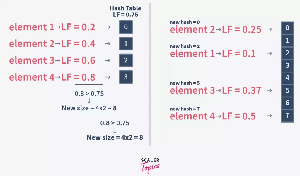
As we can see from the above,

Initialcapacity = 5
Load Factor = 0.75

Element1 added, LoadFactor = 0.2, and as 0.2 < 0.75, so no need to rehash.
Element2 added, LoadFactor = 0.4, and as 0.4 < 0.75, so no need to rehash.
Element3 added, LoadFactor = 0.6, and as 0.6 < 0.75, so no need to rehash.
Element4 will have LoadFactor = 0.8, and as 0.8 > 0.75, the HashTable is rehashed.

BucketSize is doubled, and all existing elements are picked and their new hash is created and placed at new Index in newly resized Hash Table.

New size = 5 * 2 = 10.

Element4 added, LoadFactor = 0.4, after rehashing.
Element5 added, LoadFactor = 0.5, and as 0.5 < 0.75, so no need to rehash.

Supercharge Your Coding Skills! Enroll Now in Scaler Academy's DSA Course and Master Algorithmic Excellence.