Master Theorem

Master’s Theorem is the best method to quickly find the algorithm’s time complexity from its recurrence relation. This theorem can be applied to decreasing and dividing functions, each of which we’ll look into in detail.

We can apply Master’s Theorem for:

1. Dividing Functions
2. Decreasing Functions

Master Theorem for Dividing Functions

Highlights:

• Used to directly calculate the time complexity function of ‘dividing’ recurrence relations of the form:
• $T(n)$ = $aT(n/b)+f(n)$
• where $f(n)$ = $\theta (n^{k}lo{g}^{p}n)$
• Compare $lo{g}_{b}a$ and $k$ to decide the final time complexity function.

Master's Theorem is the most useful and easy method to compute the time complexity function of recurrence relations.
Master's Algorithm for dividing functions can only be applied to the recurrence relations of the form:
$T(n)$ = $aT(n/b)+f(n)$,
where $f(n)=\theta (n^{k}lo{g}^{p}n)$
for example:

• $T(n)$ = $2T(n/2)$ + $n^2$
• $T(n)$ = $T(n/4)$ + $nlogn$

where,

n = input size (or the size of the problem)
a = count of subproblems in the dividing recursive function
n/b = size of each subproblem (Assuming size of each subproblem is same)

Where the constants a, b, and k are constants and follow the following conditions:

1. a>=1
2. b>1
3. k>=0

$T(n)=aT(\frac{n}{b})+\theta (n^{k}lo{g}^{p}n)$

Master's Theorem states that:

• Case 1) If $lo{g}_{b}a>k$ then:
• $T(n)$ = θ$(n^{lo{g}_{b}a})$
• Case 2) If $lo{g}_{b}a=k$, then:
• a) If p>-1, then $T(n)$ = $\theta (n^{k}lo{g}^{(p+1)}n)$
• b) If p=-1, then $T(n)$ = $\theta (n^{k}loglogn)$
• c) p<-1, then $T(n)$ = $\theta (n^k)$
• Case 3) If $lo{g}_{b}a<k$, then:
• If p>=0, then $T(n)$ = $\theta (n^{k}lo{g}^{p}n)$
• If p<0, then $T(n)$ = $\theta (n^k)$

The same can also be written as:

• Case 1– If $a>b^k$, then:
• $T(n)$ = θ$(n^{lo{g}_{b}a})$
• Case 2– If $a=b^k$, then:
• a) If p>-1, then $T(n)$ = θ$(n^{lo{g}_{b}a}lo{g}^{p+1}n)$
• b) If p=-1, then $T(n)=\theta (n^{lo{g}_{b}a}loglogn)$
• c) If p<-1, then $T(n)=\theta (n^{lo{g}_{b}a})$
• Case 3– If $a<b^k$, then:
• a) If p>=0, then $T(n)=\theta (n^{k}lo{g}^{p}n)$
• b) If p<0, then $T(n)=\theta (n^k)$

Hence, using the values of a, b, k and p, we can easily find the time complexity function of any dividing recurrence relation of the above-stated form. We’ll solve some examples in the upcoming section.

Examples of Master Theorem for Dividing Function

We’ll now solve a few examples to understand Master’s Theorem better. Before solving these examples, remember:

Master's Theorem can solve ‘dividing’ recurrence relations of the form $T(n)=aT(n/b)+f(n)$,
where $f(n)=\theta (n^{k}lo{g}^{p}n)$

Where the constants a, b, and k follow the following conditions:

• a>=1
• b>1
• k>=0

Example 1: $T(n)=T(n/2)+n^2$

After comparison,
a = 1, b = 2, k = 2, p = 0, $f(n)=n^2$

• Step 1: Calculate $lo{g}_{b}a$ and k
• $lo{g}_{b}a=lo{g}_{2}1=0$
• k = 2,
• Step 2: Compare with k
• $lo{g}_{b}a<k$ (Case III)
• Step 3: Calculate time complexity
• If $p>=0$, then $T(n)=\theta (n^{k}lo{g}^{p}n)$
• $T(n)=\theta (n^{2}lo{g}^{0}n)$
• $T(n)=\theta (n^2)$

Final Time complexity: $\theta (n^2$)

Example 2: $T(n)=2T(\sqrt{n})+\log n$

This recurrence relation function is not of the form $aT(n/b)+f(n)$ but can be converted to this form and then solved with Master’s Theorem. Let us convert the function form:

Let $logn=m=>n=2^m$

On replacing $n$ with $2^m$ everywhere, we get:

$T(2^m)=2T(2^{m/2})+m$
Suppose $T(2^m)=S(m)$
=> $S(m)=2S(m/2)+m$
Finally ,we have this equation of the form T(n) = aT(n/b) + f(n), where a = 2, b = 2, k = 1, p = 0, and f(m) = m

• Step 1: Calculate $lo{g}_{b}a$ and k
• $lo{g}_{b}a=lo{g}_{2}2=1$
• k = 1,
• Step 2: Compare with k
• $lo{g}_{b}a=k$ (Case II)
• Step 3: Calculate time complexity*
• If p>-1, then $T(m)=\theta (m^{k}lo{g}^{p+1}m)$
• $T(m)=\theta (m^{1}lo{g}^{1}m)$
• $T(m)=\theta (mlogm)$
• Step 4: Replacing m with $T(2^n)$

Final Time complexity: $\theta (n^2)$

Master Theorem for Decreasing Functions

Highlights:

• Used to directly calculate the time complexity function of ‘decreasing’ recurrence relations of the form:
• $T(n)$ = $aT(n-b)$ + $f(n)$
• $f(n)$ = $\theta (n^k)$
• The value of ‘a’ will decide the time complexity function for the ‘decreasing’ recurrence relation.

For decreasing functions of the form $T(n)=aT(n-b)+f(n)$,
where $f(n)$ = $\theta (n^k)$
for example:

• $T(n)=T(n-2)+1$
• $T(n)=2T(n-1)+n^2$

Where:
n = input size (or the size of the problem)
a = count of subproblems in the decreasing recursive function
n-b = size of each subproblem (Assuming size of each subproblem is same)

Here, a, b, and k are constants that satisfy the following conditions:

• a>0, b>0
• k>=0

Case 1) If a<1, then $T(n)=\theta (n^k)$

Case 2) If a=1, then $T(n)=\theta (n^{k+1})$

Case 3) If a>1, then $T(n)=\theta (n^{\frac{n}{b}}\ast f(n))$

Hence, given a decreasing function of the above-mentioned form, we can easily compare it to the given form to get the values of a, b, and k. We can find the time complexity function by looking at the three cases mentioned above. We’ll solve some examples in the upcoming section to understand better.

Examples of Master Theorem for Decreasing Function

We can solve ‘decreasing’ functions of the following form using ‘Master’s Theorem for Decreasing Functions’.
Form: T(n) = aT(n-b) + f(n),
where f(n) = θ(n^k)

Here, a, b, and k are constants that satisfy the following conditions:

• a>0, b>0
• k>=0

Example 1:

$T(n)=2T(n-2)+n$
After comparison,
$a=2,b=2,k=1,f(n)=n$

• Step 1: Compare ‘a’ and 1
• Since a>1,
• $T(n)=\theta (a^{\frac{n}{b}}\ast f(n))$
• Step 2: Calculate time complexity
• Putting values of a = 2, b = 2, f(n) = n.
• $T(n)=\theta (2^{\frac{n}{2}}\ast n)$

Final Time complexity: $\theta (2^{\frac{n}{2}}\ast n)$

Example 2:

$T(n)=1/2T(n-1)+n^2$
After comparison,
a = 1/2, b = 1, k = 2, $f(n)=n^2$

• Step 1: Compare ‘a’ and 1
• Since $a<1$,
• $T(n)$ = θ(a^k)
• Step 2: Calculate time complexity
• Putting values of a = 2,and k = 2.
• $T(n)=\theta (n^2)$

Final Time complexity: θ(n^2^)

Idea Behind Master Theorem for Dividing Functions

Highlights:

• To calculate $lo{g}_{b}a$ and compare it with $f(n)$ to decide the final time complexity of the recurrence relation $T(n)$

The idea behind Master's algorithm is based on the computation of $n^{logba}$ and comparing it with $f(n)$. The time complexity function is the one overriding the other.

For Example:

• In Case I, $n^{logba}$ dominates $f(n)$. So the time complexity function $T(n)$ comes out to be $\theta (n^{logba})$
• In Case II, $n^{logba}$ is dominated by $f(n)$. Hence, the $f(n)$ function will take more time, and the time complexity function, in this case, is $\theta (f(n))$, i.e., $\theta (n^{k}lo{g}^{p}n)$.
• In case III, when $lo{g}_{b}a=k$, the time complexity function is going to be $\theta (n^{logba}logn)$

Now, Why do We Compare $n^{logba}$ with $f(n)$ and not Some Other Computation?

Given $T(n)$ = $aT(n/b)$ + $f(n)$, we need to calculate the time complexity of $T(n)$. Suppose we calculate the time taken by both the terms individually and compare which one dominates. In that case, we can easily define the time complexity function of $T(n)$ to equal the one that dominates.

To achieve this, let’s first understand the first term, i.e., $aT(n/b)$, and then, we will calculate the time taken by this term.

Understanding the Term – $aT(n/b)$
$aT(n/b)$ means – For our problem of size n, we divide the whole problem into 'a' subproblems of size 'n/b' each. Suppose $T(n)$^’^ is the time taken by the first term.

Hence,
=> $T(n{)}^{‘}=aT(n/b)$
$T(n/b)$ can again be divided into sub problems of size $(n/b^2)$ each.

Hence,
=> $T(n{)}^{‘}=aT(n/b)=a^{2}T(n/b^2)$
Similarly,
=> $T(n{)}^{‘}=a^{3}T(n/b^3)$ and so on.
to
=> $T(n{)}^{‘}=a^{i}T(n/b^i)$

Let’s assume $n=b^k$ (When we divide a problem to 1/2 each time, we can say that $n=2^k$. Here we divide the problem with b each time,, hence, $n=b^k$)
=> $n=b^k$
=> $lo{g}_{b}n=k$

At the ith level, the size of the sub-problem will reduce to 1, i.e. at the ith level,

=> $n/b^i=1$
=> $n=b^i$
=> $lo{g}_{b}n=i=k$,
Therefore, i = k at the last level, where the size of the sub-problem reduces to 1.

Using this deduction, we can re-write $T(n{)}^{‘}$ as:

=> $T(n{)}^{‘}=a^{i}T(n/b^i)$
=> $a^{logbn}T(b^i/b^i)$
=> $a^{logbn}T(1)$
Hence, $T(n{)}^{‘}=\theta (a^{logbn})=\theta (n^{logba})$

$T(n{)}^{‘}$ was assumed to be the time complexity function for the first term. Hence proved that the first term takes $n^{logba}$ time complexity. That is why we compare $n^{logba}$ (i.e. the first term) with f(n) (i.e. the second term) to decide which one dominates, which decides the final time complexity function for the recurrence relation.

Proof of Master Algorithm

$T(n)=a\ast T(\frac{n}{b})+O(n^d)$

This form of recurrence relation is in the form of a tree, as shown below, where every iteration divides the problem into ‘a’ sub-problems of size (n/b).

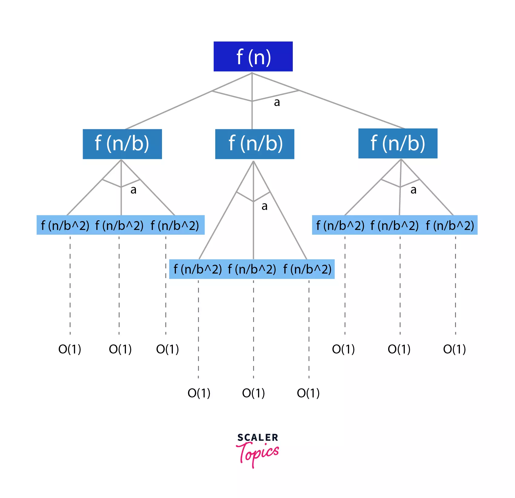
At the last level of the tree, we will be left with problems of size 1. This is the level where we have the shortest possible sub-problems.

The level = $lo{g}_{b}n$
Size of sub-problem = 1

Let us now calculate the work done at each level and that will help us compute the total work done, i.e. the sum of work done at log~b~n levels.

• Work done at level 1 => $O(n^d)$
  n^d^ comes from the recurrence relation
• Work done at level 2 => $a\ast O(n/b^d)$ => $a/b^d\ast O(n^d)$
  At the second level, the problems are divided into size n/d, and there are ‘a’ sub-problems.
• Work done at level k => $(a/b^d{)}^k\ast O(n^d)$
• Hence, Total Work Done => ${\Sigma }_{k=0}^{lo{g}_{b}n}(a/b^d{)}^k\ast O(n^d)$.

Note: This Summation forms a Geometric Series.

Now, let us look at every single case and prove it.

Proof of Case I: When $d<lo{g}_{a}b$

• In this case, the work done increases as we move down the tree, i.e. towards the lower levels of the tree, with more sub-problems.
• Also, the total work done is an expression of the Geometric Series, and in this case, r<1. Hence, the last term of the geometric series will have the maximum effect.
• Hence, the total work done will only include the last term since all the other terms of the geometric series can be ignored compared to the last one.
• Hence, we can substitute k = log~b~n in the time complexity expression.

=> $O(O(n^d)(\frac{a}{b^d}{)}^{lo{g}_{b}n})$
=> $O(O(n^d)\frac{a^{lo{g}_{b}n}}{b^{d}lo{g}_{b}n})$
=> $O(O(n^d)\frac{n^{lo{g}_{b}a}}{n^d})$
=> $O(n^{lo{g}_{b}a})$

Proof of Case II: When $d=lo{g}_{a}b$

• This means that the work done by each term in the geometric series is equal.
• Hence, the total work is work done at each level * Number of levels.

=> $O(\sum _{i=0}^{lo{g}_{b}n}O(n^d))$
=> $(1+lo{g}_{b}n)O(n^d)$
=> $O(n^{d}logn)$

Proof of Case III: When $d>lo{g}_{a}b$

• This is exactly the opposite of the first case discussed.
• This is the case of decreasing Geometric Series. Hence, the first term is the maximum and major term to be considered.
• Hence, the total work done = first term, i.e. O(n^d^)

Hence, Proved!

Limitations of Master Theorem in DAA

Highlights:

The relation function cannot be solved using Master's Theorem if:

• T(n) is a monotone function
• a is not a constant
• f(n) is not a polynomial

Master's Theorem can only be used for recurrence relations of the form:

• $T(n)$ = $aT(n/b)$ + $f(n)$, where $f(n)=\theta (n^{k}lo{g}^{p}n)$ (Dividing Recurrence Relation)
  Or,
• $T(n)$ = $aT(n-b)$ + $f(n)$, where $f(n)=\theta (n^k)$ (Decreasing Recurrence Relation)

This marks the limitations of Master's Theorem, which cannot be used if:

• T(n) is monotone function, For example: $T(n)$ = $cosx$
• a is not a constant. Consider this: $T(n)$ = $nT(n/3)+f(n)$. This function cannot be solved to get the time complexity functions because that changes our comparison function(as discussed above). We compare $n^{logba}$ with $f(n)$ for the final dominating time function.

If a is not constant, this changes our Master Theorem's conditions altogether.

• If $f(n)$ is not a polynomial. Again, for similar reasons, the Master's Theorem can only be applied to the above-stated form under the given constraints.

Conclusion

• We learn the master theorem for dividing and decreasing functions.
• For the recurrence relations of the type
  • $T(n)=aT(n/b)+f(n)$, where $f(n)=\theta (n^{k}lo{g}^{p}n)$ (Dividing Recurrence Relation)
    Or,
  • $T(n)=aT(n-b)+f(n)$, where $f(n)=\theta (n^k)$ (Decreasing Recurrence Relation)

Furthermore, our online DSA course delves deep into the Master Theorem, providing comprehensive coverage to ensure a thorough understanding.

Read More:

• Divide and Conquer