Maximum Flow and Minimum Cut

Introduction

In our previous articles, we have seen how costly it is to calculate the maximum flow as well as the minimum cut of a graph. If we want to calculate both of them, then we need not follow the conventional method to calculate them instead we will bother about calculating only one of them.

In this article, we will discuss how we can find the maximum flow of a flow network by calculating the minimum cut of the network or vice-versa. We have already seen what do minimum cut and maximum flow means in previous articles, though we have given a slight glimpse for revision of the concept.

There is a theorem that can be proved to pose a relation between maximum flow and minimum cut of a network and that theorem is known as the "Max-flow Min-cut" theorem which has been briefly explained and proved in the article.

Let's revisit the concepts of minimum cut and maximum flow and then we will see what does the max-flow min-cut theorem states and how we can prove it.

Minimum Cut Problem

Let us assume for some reason we want to split any given image into two non-similar portions. If we approach this problem in terms of graph data structure we would consider pixels as the vertices of the graph and edges between two similar pixels of the image. In this case, a minimum cut will be analogous to the partition of pixels into two parts where the two parts are the most dissimilar.

To understand the minimum cut (or simply min-cut) concept, we will take the help of an example a simple undirected graph $G$ with five vertices and six edges as shown below -

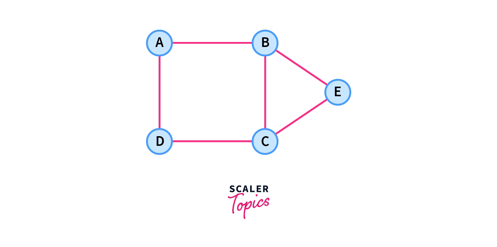
To obtain the minimum cut of this graph, we will be interested in disconnecting this graph into two components by removing the minimum possible number of edges. This can be done by removing two edges, $A\leftrightarrow B$ and $D\leftrightarrow C$ as shown below.

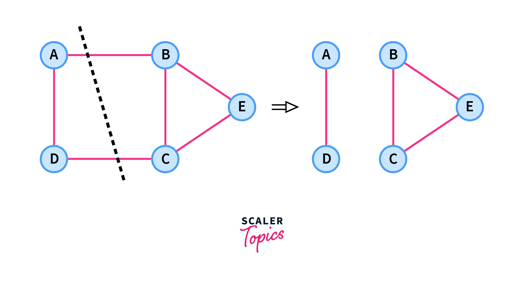
Formally minimum cut is defined as, the minimum sum of weight of the edges (minimum edges in case of unweighted graphs) required to remove to disconnect the graph into two components.

Karger's algorithm is a randomized algorithm that is used to find the minimum cut of any given graph $G$ has been discussed in the Minimum cut article. We would strongly recommend you to refer it to have an idea of its implementation.

Maximum Flow Problem

If we consider a rail network that connects two cities (say $A$ and $B$) by way of several intermediate cities, where each railway line has some value assigned to it denoting its capacity.

Assuming steady conditions (number of trains on a railway line never exceeds its capacity), if we need to find what is the maximum number of trains (maximum flow) that we can send from City $A$ to city $B$ then the problem is known as the "Maximum Flow Problem".

In graph theory, we have been given a network with a source (which has no incoming edge) node and a sink (which has no outgoing edge) node and capacities of all the edges which correspond to the maximum flow that an edge can allow to flow through it.

We are interested in finding the maximum amount of flow we can send from the source node to the sink node constrained with the capacities of all the intermediate edges. To understand it more clearly we will have a look on an example have been given below -

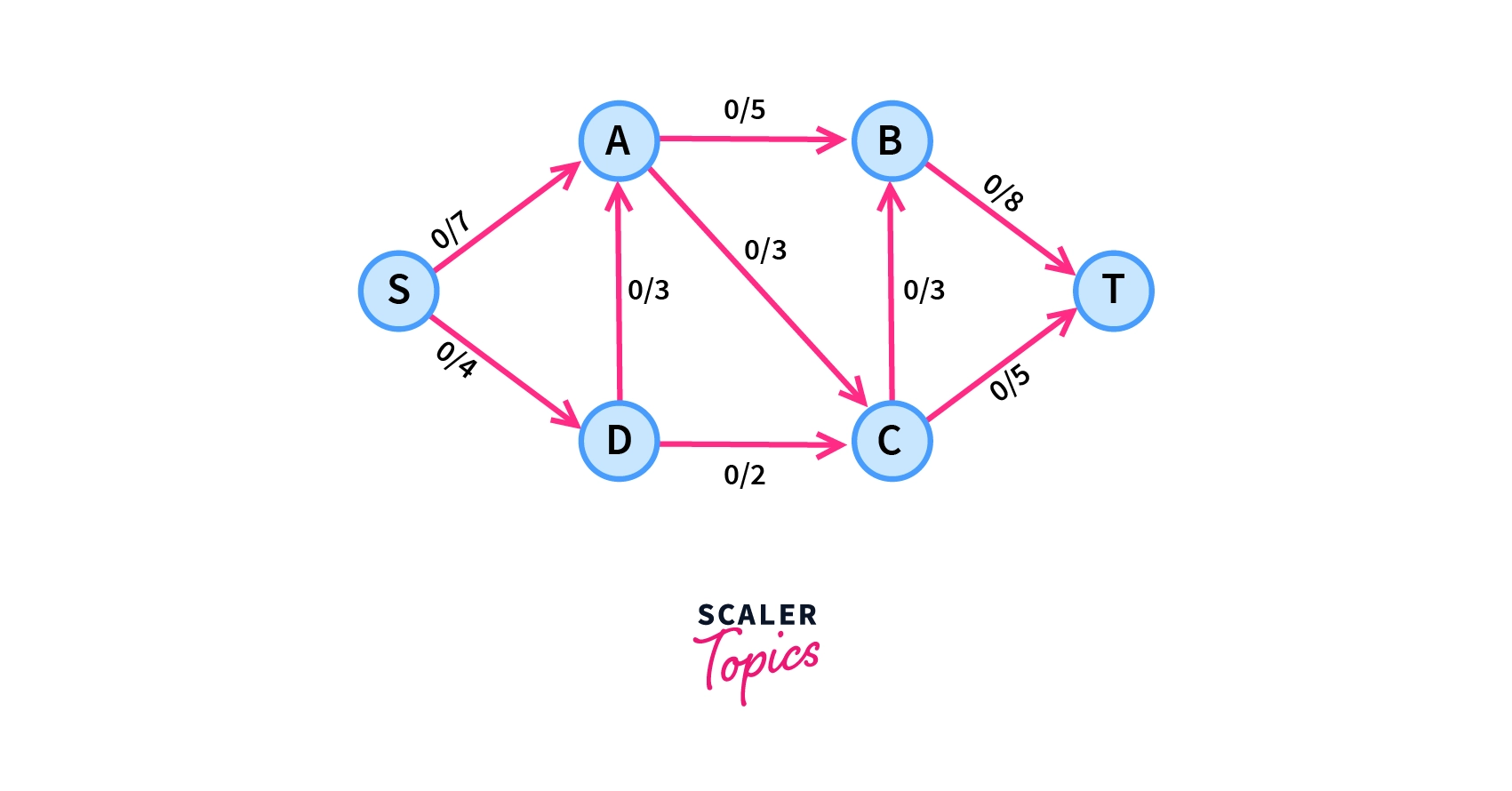
The given graph $G$ has six vertices and nine edges where the first value of each edge represents the flow through it (which is initially set to 0) and the second value represents its capacity.

For example - $0/5$ is written over edge $A\leftrightarrow B$ means capacity of this edges is 5 and currently there is no flow along this edge.

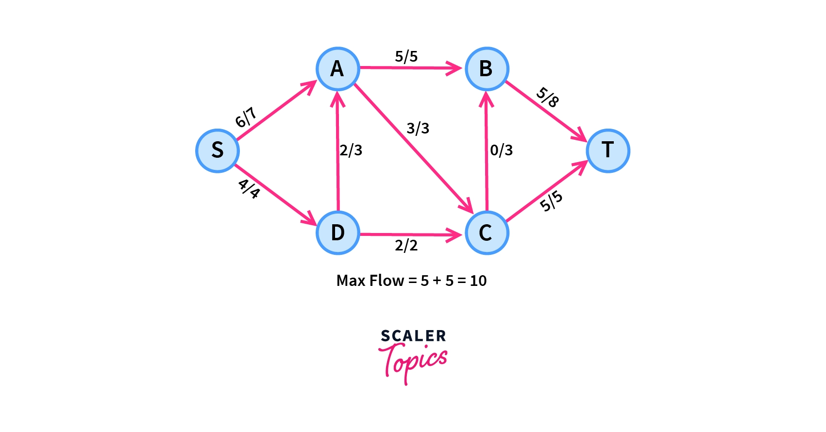
We can find the maximum flow through this network by following the steps which have been explained briefly in Maximum Flow.

After proceeding through the steps, we find maximum flow through the network as -

Max Flow Min Cut Theorem

The max-flow min-cut theorem is the network flow theorem that says, maximum flow from the source node to sink node in a given graph will always be equal to the minimum sum of weights of edges which if removed disconnects the graph into two components $i.e.$ size of the minimum cut of the graph .

More formally, the max-flow min-cut theorem states that, the maximum flow passing from the source node to the sink node is equal to the size of the minimum cut.

Intuition

In all types of networks (whether they carry data or some other object), the amount of flow that can flow through the network is restricted by the weakest connection (an edge with comparatively less capacity) between disjoint sets of the network. Even if other connections can allow a huge amount of flow through them but can never be used.

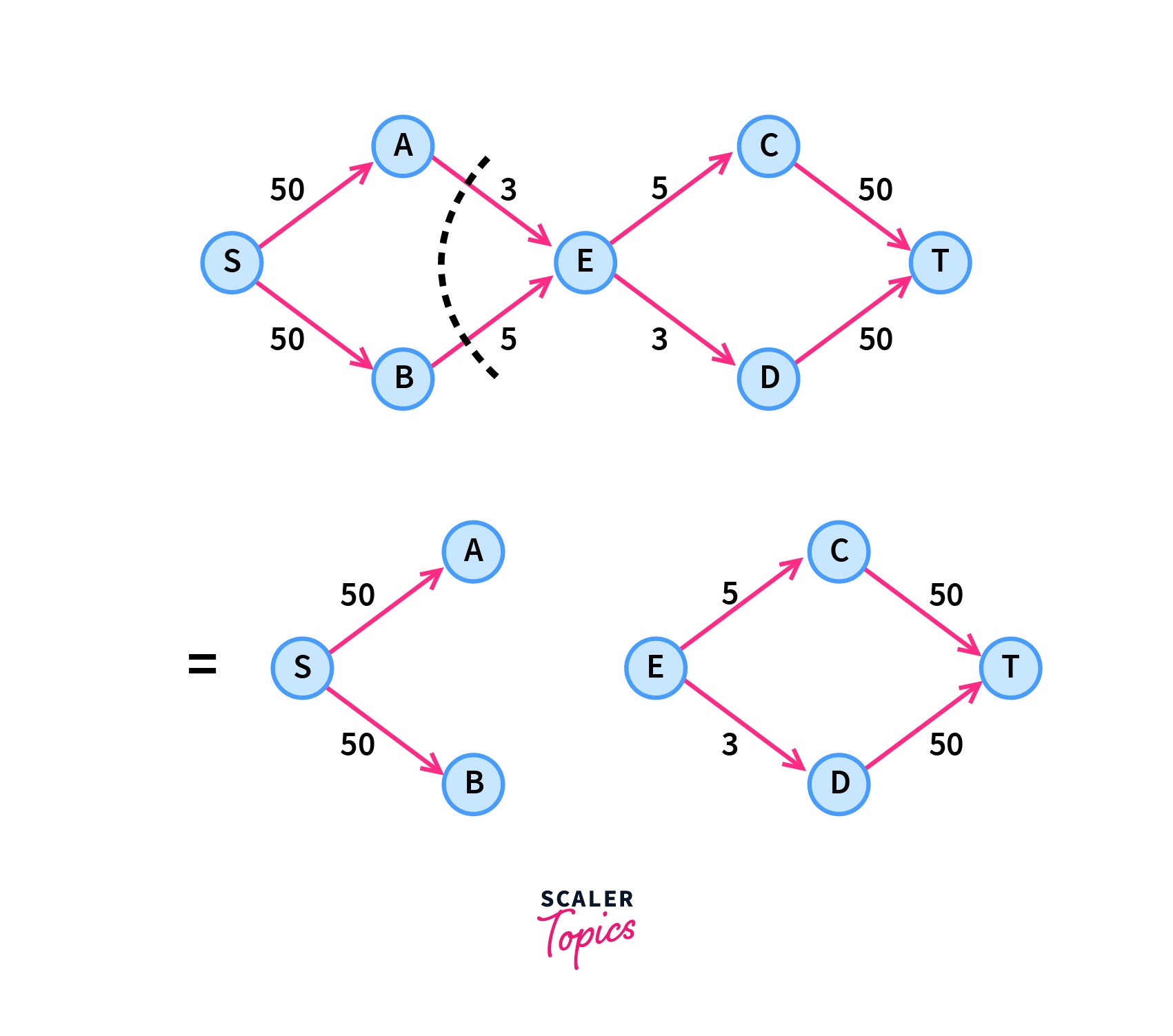
Let's have a look at an example to understand this clearly -

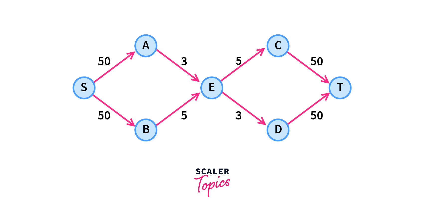
In the above-shown network, edge $s\rightarrow A, \space s\rightarrow B$ has a capacity of 50 units but we can't send that much flow through them because in the later stage we have edges $A\rightarrow B \space and \space B\rightarrow E$ with capacities of 3 and 5 respectively. Hence, the maximum flow we can have through this graph is only 8.

Another important observation in this graph is the size of the minimum cut is also 8, which can be obtained by removing edges $A\rightarrow E \space and \space B\rightarrow E$ with the total sum of weights as 8 as shown below -

Proof of Max-Flow Min-Cut Theorem

Before beginning with the proof let's define some variables which we will use frequently while proving the max-flow min-cut theorem - $G$ - The given network. $S$ - Set that includes the source node $s$. $T$ - Set that includes the sink node $t$. $f$ - A function represent flow through the network. $f^*$ - Function $f$ at its max value (Maximum flow).

Lemma - A statement that is assumed to be true and used as a basis to draw a conclusion.

Corollary - A statement which is direct result of a fact (in our case result of a Lemma).

Lemma 1:

For any flow through $f(G)$ and cut $(S,T)$ in a network, we can say that -

$f(G)\leq capacity(S,T)$

This lemma also makes sense as we have seen in the above intuition, it is not possible to send more flow through an edge than its capacity.

Corollary 2:

Because of lemma 1, for maximum flow $f(G)^*$ and minimum cut $(S,T)^*$ we have -

$f(G)^* \leq capacity((S,T)^*)$

The above mathematical result places an upper bound for the maximum flow through the graph.

According to the "Ford-Fulkerson method" let the initial flow $f$ be $0$. Now we will search for an augmenting path between $s$ and $t$ in the residual graph which has been formed at each step of the process. Let in an augmenting path $p$ from $s$ to $t$, $c_{min}$ is the minimum capacity of any edge along the path.

So we will add this flow ($c_{min}$) in our maximum flow $f^*$ -

$f^*=f+c_{min}$

This process is repeated until there are more augmenting paths in the residual network. Once there is no augmenting path left, we denote all vertices which are reachable from the source as $V$ and all vertices which are not reachable from the source as $V'$. It is obvious that sink $t$ can't be in set $V$ as there are no more paths between $s$ and $t$.

For any pair of vertices, $u \space and \space v$ where $u$ is in set $V$ and $v$ is in set $V'$. The flow $f(u,v)$ is maximized as no augmenting paths are left also flow of $(v,u)$ is 0 due to same reason.

Therefore we can say that,

$f(u,v)=capacity(u,v), \space \space \space \space u\space \epsilon \space V, \space v \space \epsilon \space V'$

And by corollary 2 we can conclude that -

$f^*=capacity((S,T)^*)$

Applications

• Generalized max-flow min-cut theorem

  If we define the capacity of vertices along with edges in a flow network. Then, flow along a path also needs to satisfy the capacity constraint of vertices $i.e.$ a flow passing through a particular vertex can't exceed its capacity. In this case, the capacity of a cut is the sum of the capacities of edges and vertices present in it.

So using this we can pose a generalized max-flow min-cut theorem will state that maximum $s-t$ flow is equal to the minimum capacity of a $s-t$ cut in a different sense to solve other complex problems.

• Project Selection Problem

  In the project selection problem, we have $p$ projects and $m$ machines. For completing a project successfully we require some machines for each project (a machine can also be shared for completing several projects), on completing each project $p_i$ we earn a revenue of $r(p_i)$, and each machine $m_j$ costs $c(m_j)$.

  We want to choose projects such that the revenue we get at the end is maximized. So we define a dummy source node $s$ connected the projects with capacity $r(p_i)$ and a dummy sink node $t$ which is connected by all the machines with capacities $c(m_j)$ also an edge is is added between $(p_i, m_j)$ if project $p_i$ requires machine $m_j$.

  Let's assume we have 3 projects and 3 machines with requirements and costs as shown in the table below -

  No.	$r(p_i)$	$c(q_j)$	$req(p_i)$
  1	50	100	$m_1 \& m_2$
  2	100	50	$m_2$
  3	75	25	$m_2 \& m_3$

  The network formed based on the data will look like -

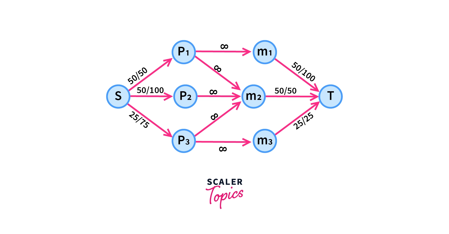
  Then one can either solve this problem with the approach used in the maximum flow problem or by finding the minimum $s-t$ cut of the network formed.

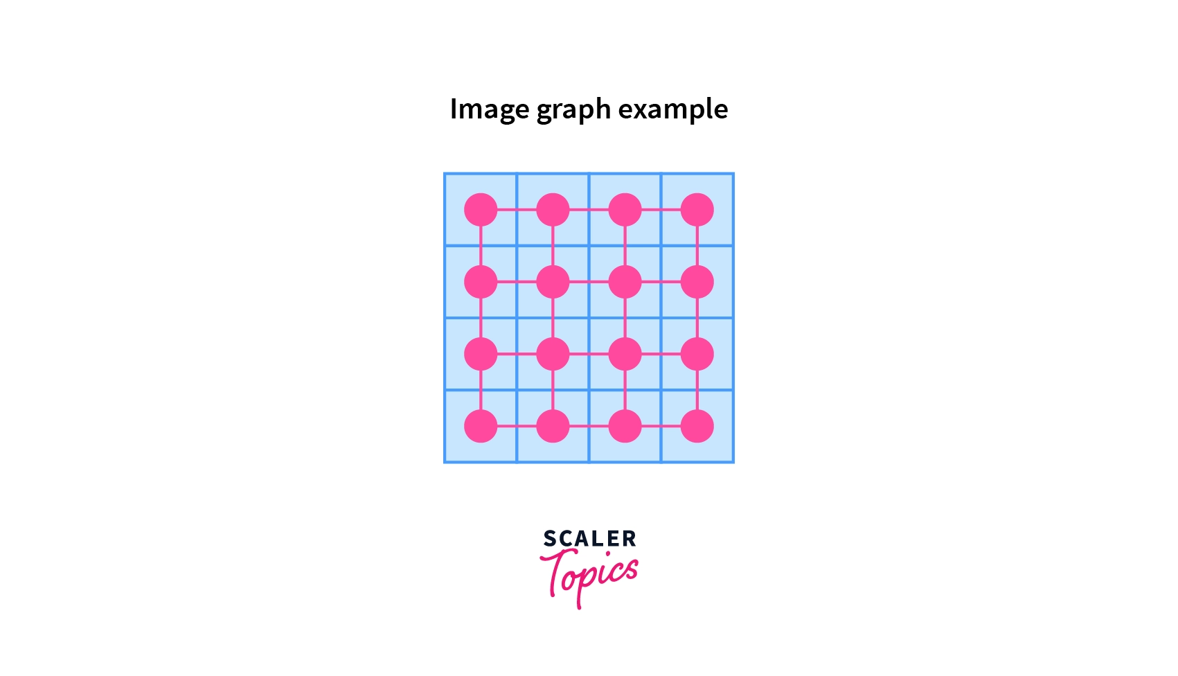
• Image Segmentation Problem

  In the image segmentation problem, we have been given an image, we want to find what is the foreground and what is the background? We have two non-negative values defined for each pixel $i$ among $n$ pixels of the given image.

  1. $f_i =$ probability that pixel $i$ is in the foreground.
  2. $b_i =$ probability that pixel $i$ is in the background.

  We will consider a pixel in the foreground if $f_i>b_i$ and background in the other case.

  In terms of graph data structure, we consider every pixel as a vertex and edge between vertex $i \space and \space j$ if they are adjacent to each other as shown below -

Now we introduce a new term penalty which we have for each adjacent pair of pixels ${i,j}$ in case one is in the foreground and other in the background.

We will define a dummy source node connected with all vertices with capacities $f_i$ and a sink node which is also connected to all the vertices with capacities $b_i$ also, edges $(i,j)$ and $(j,i)$ are added with capacity as $p_{ij}$ between two adjacent pixels.

Then the minimum s-t cut represents pixels assigned to the foreground $P$ and pixels assigned to the background in $Q$.