Open Addressing | Closed Hashing

Open Addressing, also known as closed hashing, is a simple yet effective way to handle collisions in hash tables. Unlike chaining, it stores all elements directly in the hash table. This method uses probing techniques like Linear, Quadratic, and Double Hashing to find space for each key, ensuring easy data management and retrieval in hash tables.
The main concept of Open Addressing hashing is to keep all the data in the same hash table and hence a bigger Hash Table is needed. When using open addressing, a collision is resolved by probing (searching) alternative cells in the hash table until our target cell (empty cell while insertion, and cell with value while searching ) is found. It is advisable to keep load factor () below , where is defined as where is the total number of entries in the hash table and is the size of the hash table. As explained above, since all the keys are stored in the same hash table so it's obvious that because always. If in case a collision happens then, alternative cells of the hash table are checked until the target cell is found. More formally,
- Cells are tried consecutively until the target cell has been found in the hash table. Where keeping .
- The collision function is decided according to method resolution strategy.
There are three main Method Resolution Strategies --
- Linear Probing
- Quadratic Probing
- Double Hashing
Linear Probing
In linear probing, collisions are resolved by searching the hash table consecutively (with wraparound) until an empty cell is found. The definition of collision function is quite simple in linear probing. As suggested by the name it is a linear function of or simply . Operations in linear probing collision resolution technique -
- For inserting we search for the cells until we found a empty cell to insert .
- For searching we again search for the cells until we found a cell with value . If we found a cell that has never been occupied it means is not present in the hash table.
- For deletion, we repeat the search process if a cell is found with value we replace the value with a predefined unique value (say ) to denote that this cell has contained some value in past.
Example of linear probing -
Table Size = Hash Function - Collision Resoulution Strategy -
- Insert -
- Search -
- Delete -
Steps involved are
-
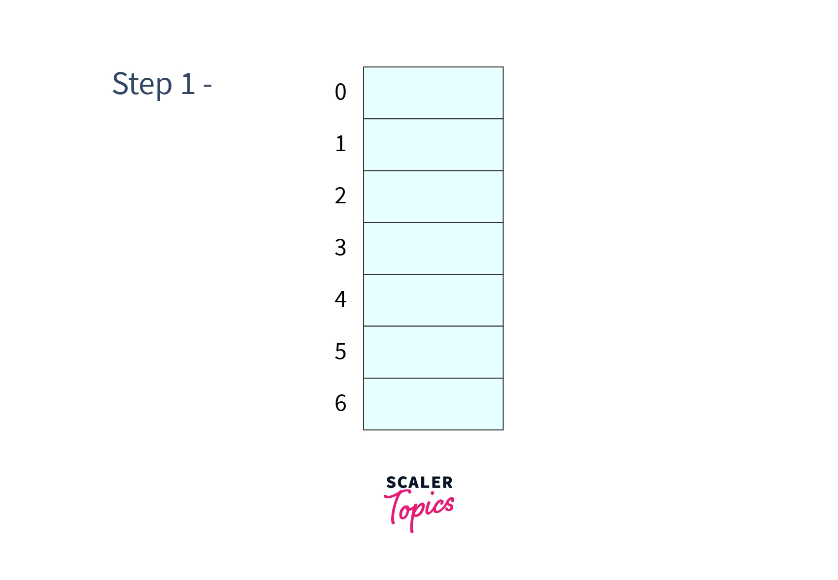
Step 1 - Make an empty hash table of size 7.
-
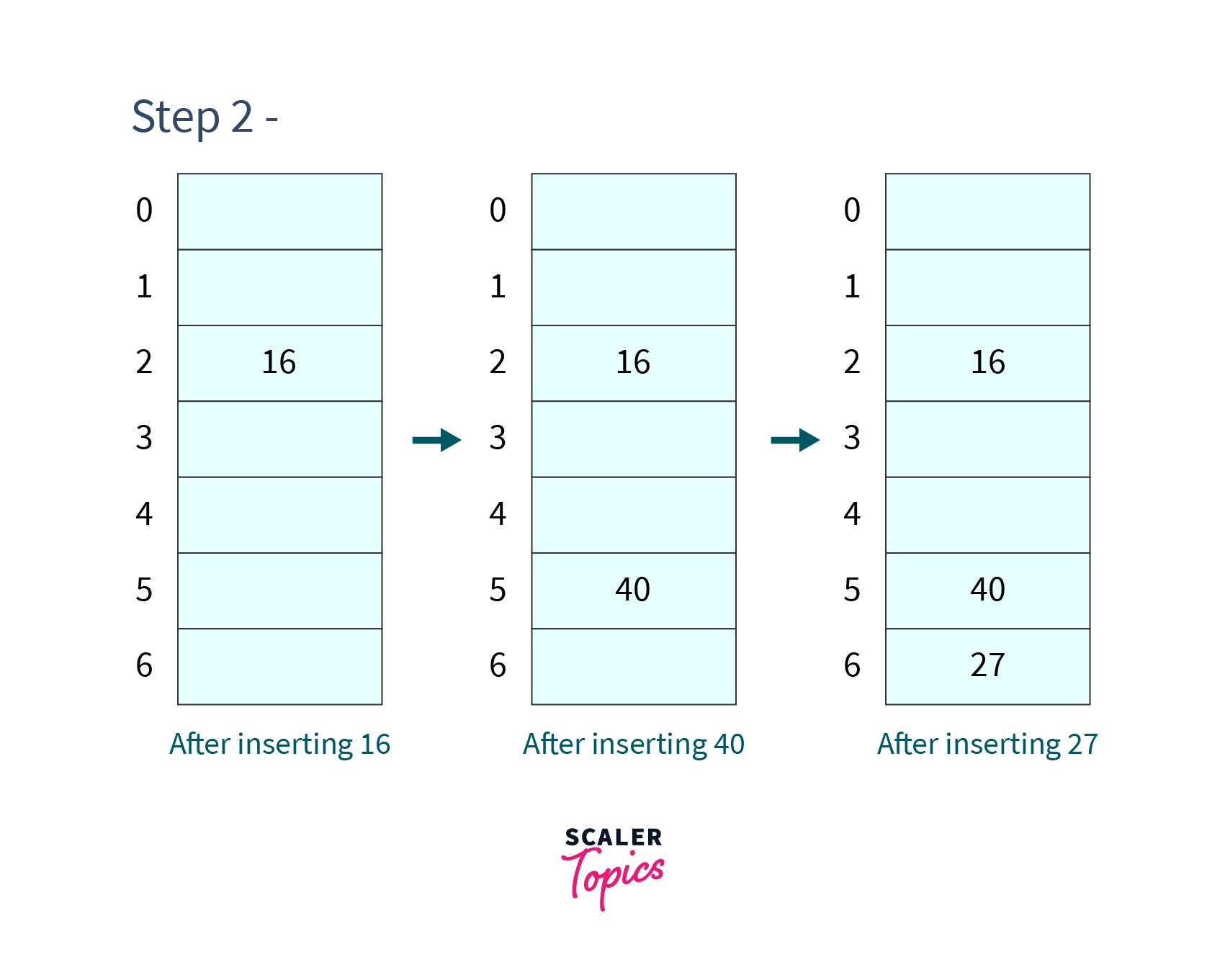
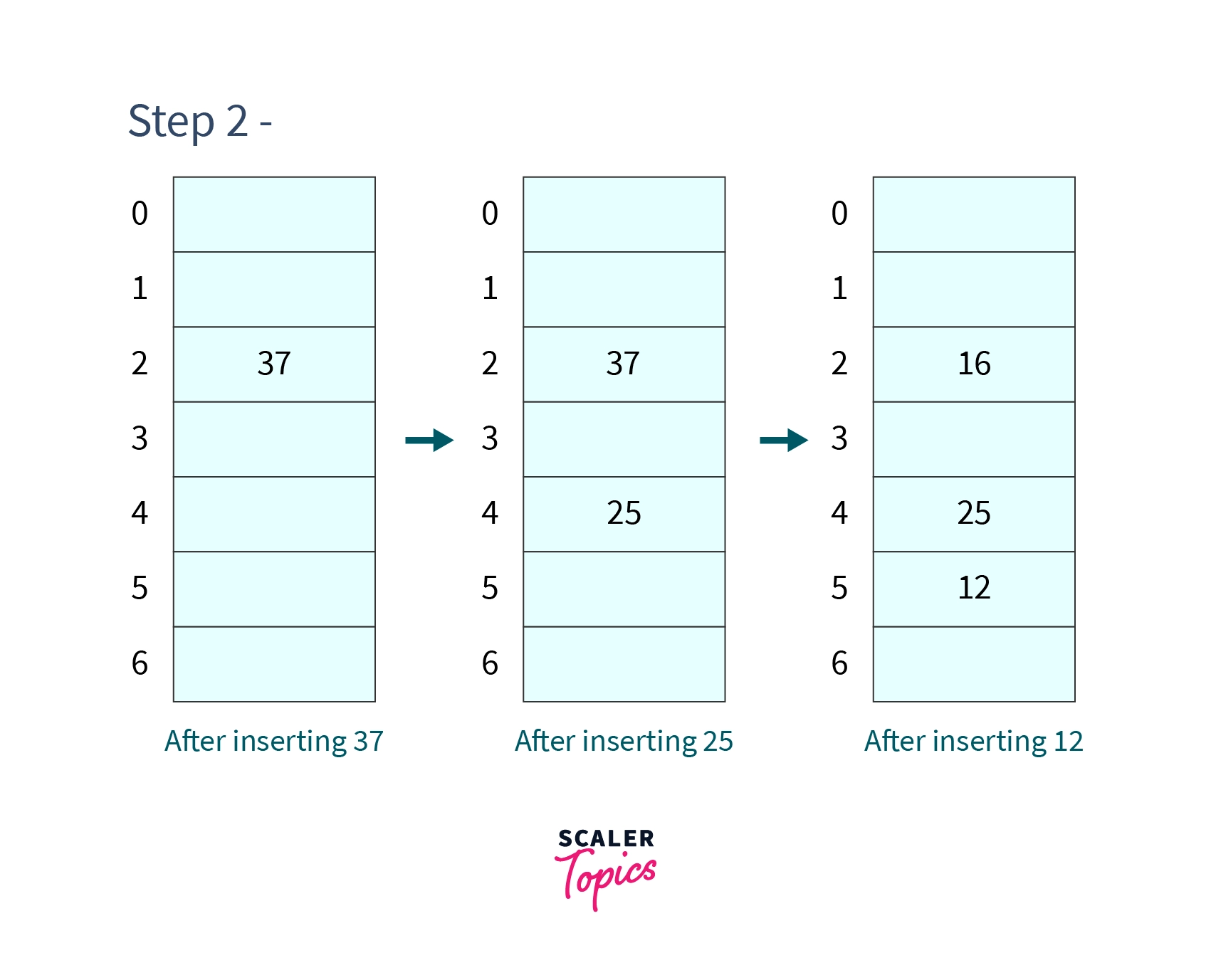
Step 2 - Inserting , and .
As we do not get any collision we can easily insert values at their respective indexes generated by the hash function.
After inserting, the hash table will look like -
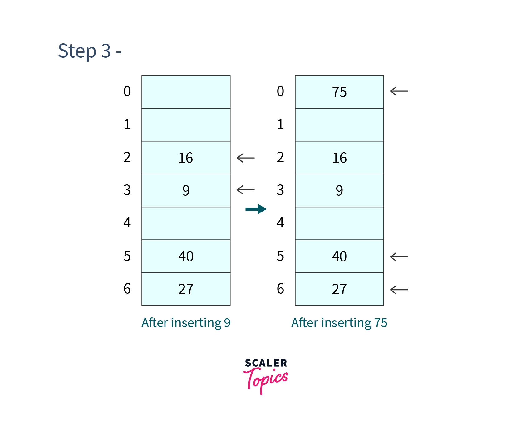
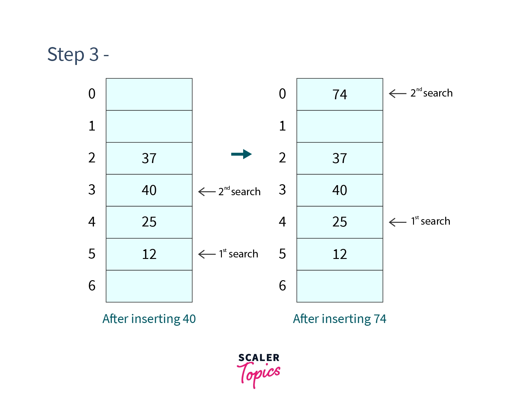
- Step 3 - Inserting 9 and 75.
-
But at index already is placed and hence collision occurs so as per linear probing we will search for consecutive cells till we find an empty cell.
So we will probe for cell 3, since the next cell is not occupied we place 9 in cell . - Again collision happens because 40 is already placed in cell . So will search for the consecutive cells, so we search for cell which is also occupied then we will search for cell which is empty so we will place 75 there.
-
But at index already is placed and hence collision occurs so as per linear probing we will search for consecutive cells till we find an empty cell.
After inserting and hash table will look like -
- Step 4 - Search and -
- But at index is not present so we search for consecutive cells until we found an empty cell or a cell with a value of . So we search in cell but it does not contain , so we search for in cell and we stop our search here as we have found .
- We will search for in cell but it contains 75 so we will search in the next cell since it is found empty it is clear that do not exist in our table.
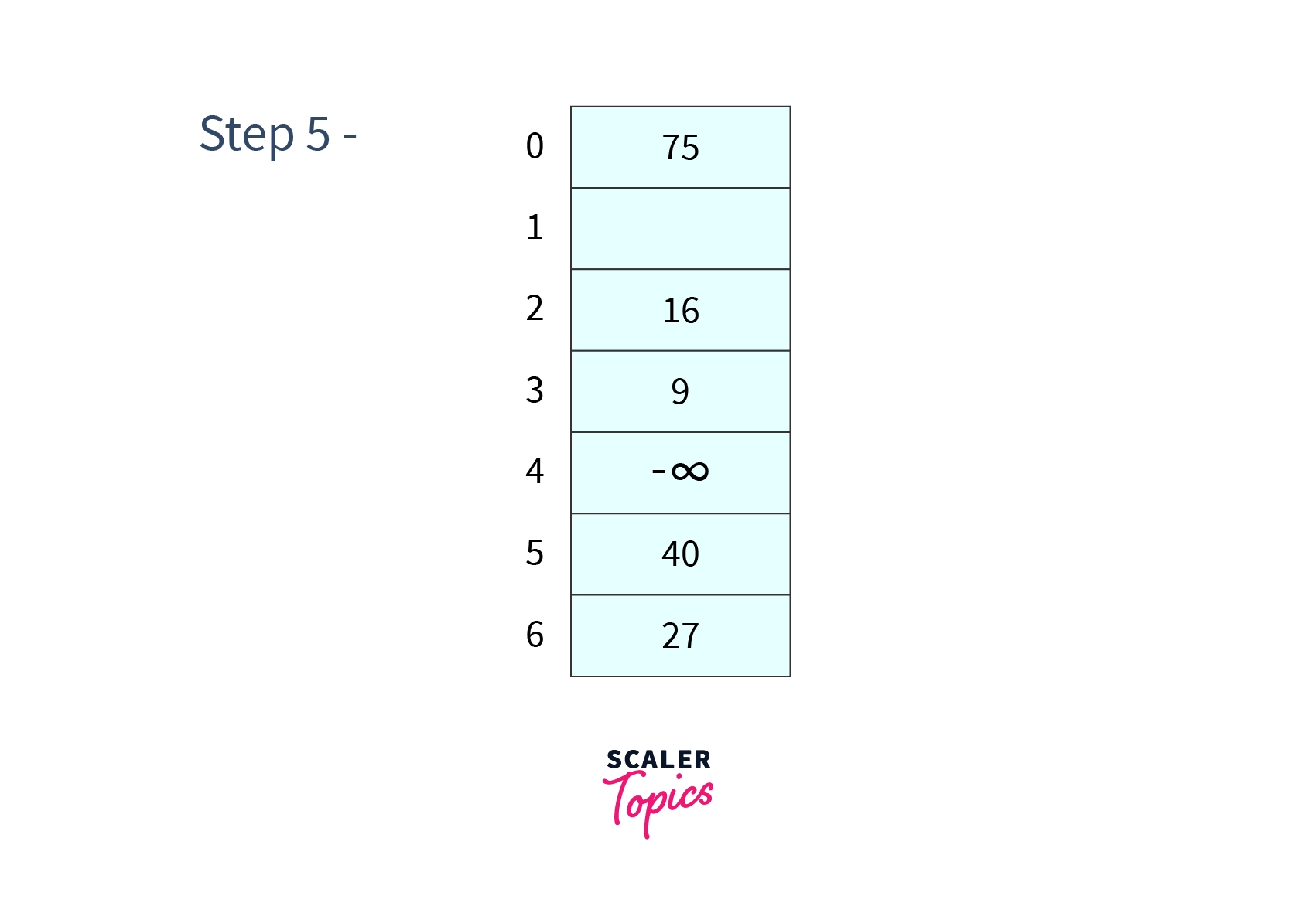
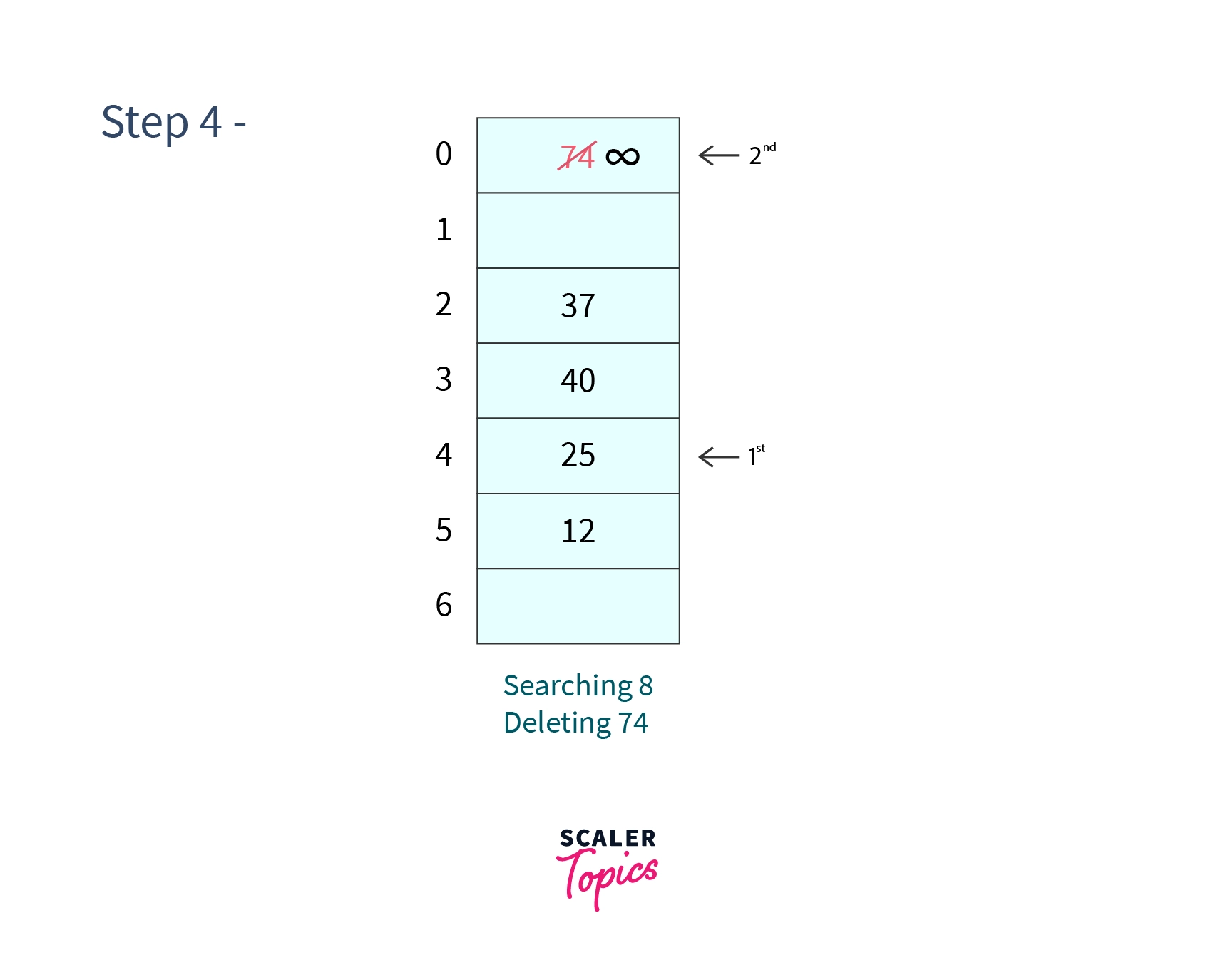
- Step 5 - Delete
- Firstly we search for which results in a successful search as we get in cell then we will remove from cell and replace it with a unique value (say -ash).
After all these operations our hash table will look like -
Algorithm of linear probing
- Insert() -
- Find the hash value, of from the hash function .
- Iterate consecutively in the table starting from the till you find a cell that is currently not occupied.
- Place in that cell.
- Search() -
- Find the hash value, of from the hash function .
- Iterate consecutively in the table starting from the till you find a cell that contains or which is never been occupied.
- If we found , then the search is successful and unsuccessful in the other case.
- Delete() -
- Repeat the steps of Search().
- If element does not exist in the table then we can't delete it.
- If exists in the cell (say ), put in cell k to denote it has been occupied some time in the past, but now it is empty.
Pesudocode of Linear Probing
Transform Your Career
Choose from our industry-leading programs designed for career success
Modern Software and AI Engineering Program
Master full-stack development with AI integration

Modern Data Science and ML with specialisation in AI
Advanced data science techniques with AI specialization
Advanced AIML with Specialisation in Agentic AI
Deep dive into AIML with focus on Agentic systems
DevOps, Cloud & AI Platform Engineering
Build and manage AI-powered cloud infrastructure
AI Engineering Advanced Certification by IIT-Roorkee
Premier AI engineering certification from IIT-Roorkee
Code of Linear Probing
- C/C++
- Java
Output -
Problem With Linear Probing
Even though linear probing is intuitive and easy to implement but it suffers from a problem known as Primary Clustering. It occurs because the table is large enough therefore time to get an empty cell or to search for a key is quite large. This happens mainly because consecutive elements form a group and then it takes a lot of time to find an element or an empty cell which ultimately makes the worst case time complexity of searching, insertion and deletion operations to be , where is the size of the table.
Quadratic Probing
Quadratic probing eliminates the problem of "Primary Clustering" that occurs in Linear probing techniques. The working of quadratic probing involves taking the initial hash value and probing in the hash table by adding successive values of an arbitrary quadratic polynomial. As suggested by its name, quadratic probing uses a quadratic collision function . One of the most common and reasonable choices for is -- Operations in quadratic probing collision resolution strategy are -
- For inserting we search for the cells until we find an empty cell to insert .
- For searching we again search for the cells until we find a cell with value . If we find an empty cell that has never been occupied it means is not present in the hash table.
- For deletion, we repeat the search process if a cell is found with value we replace the value with a predefined unique value to denote that this cell has contained some value in past.
You can see that the only one change between linear and quadratic probing is that in case of collision we are not searching in cells consecutively, rather we are interested in probing the cells quadratically. Let us understand this by an example -
Example of Quadratic Probing
Table Size = 7 Insert = 15, 23, and 85. Search & Delete = 85 Hash Function - Collision Resolution Strategy -
-
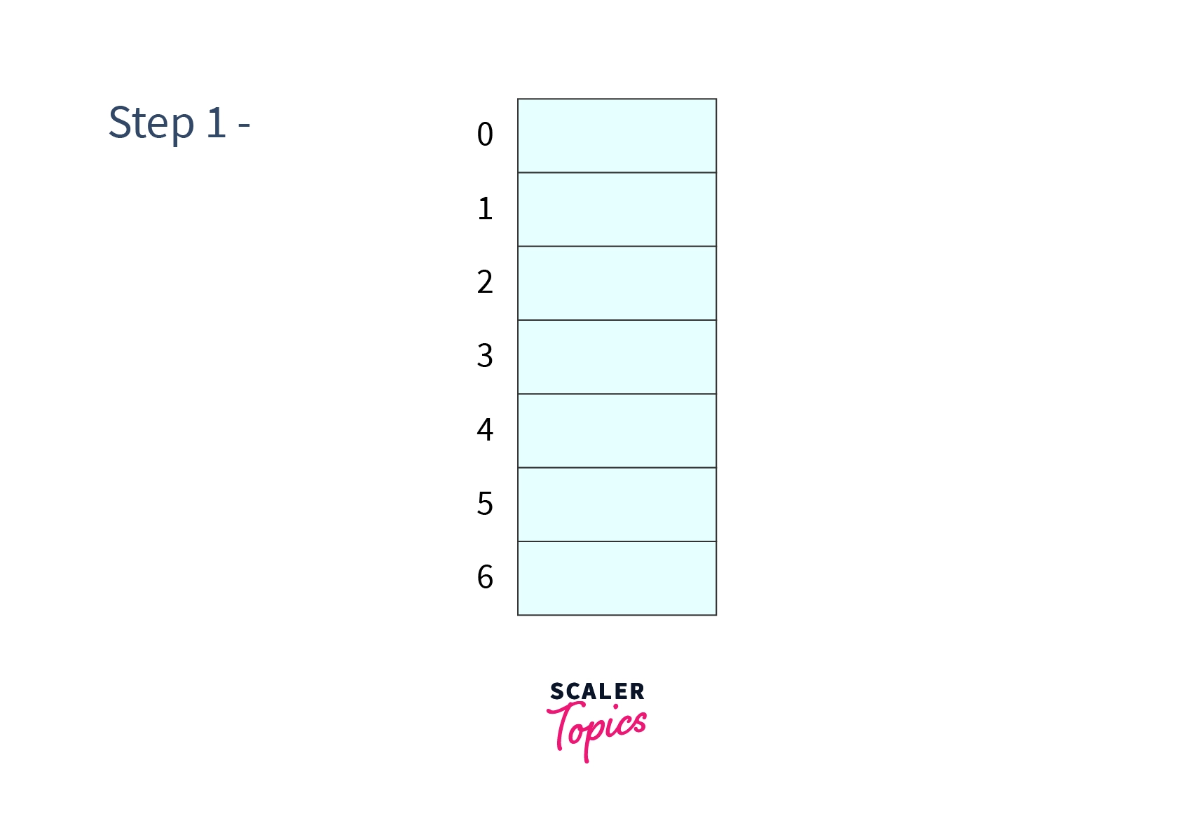
Step 1 - Create a table of size .
-
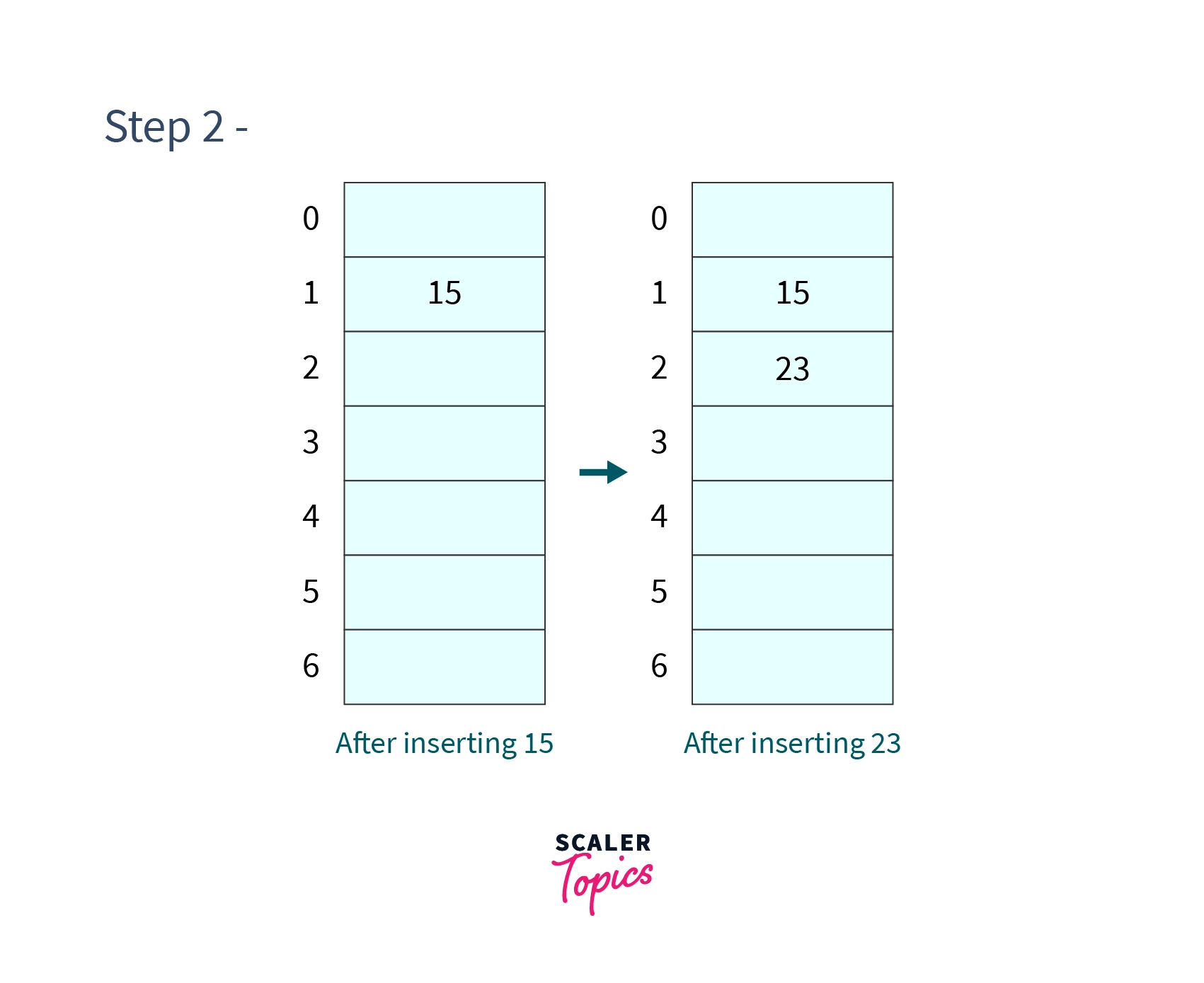
Step 2 - Insert and
- Since the cell at index 1 is not occupied we can easily insert 15 at cell 1.
-
Again cell 2 is not occupied so place 23 in cell 2.
After performing this step our hash table will look like -
-
Step 3 - Inserting
-
In our hash table cell 1 is already occupied so we will search for cell cell .
Again it is found occupied so we will search for cell cell . It is not occupied so we will place in cell .
After performing all these insertions in our hash table it will look like -
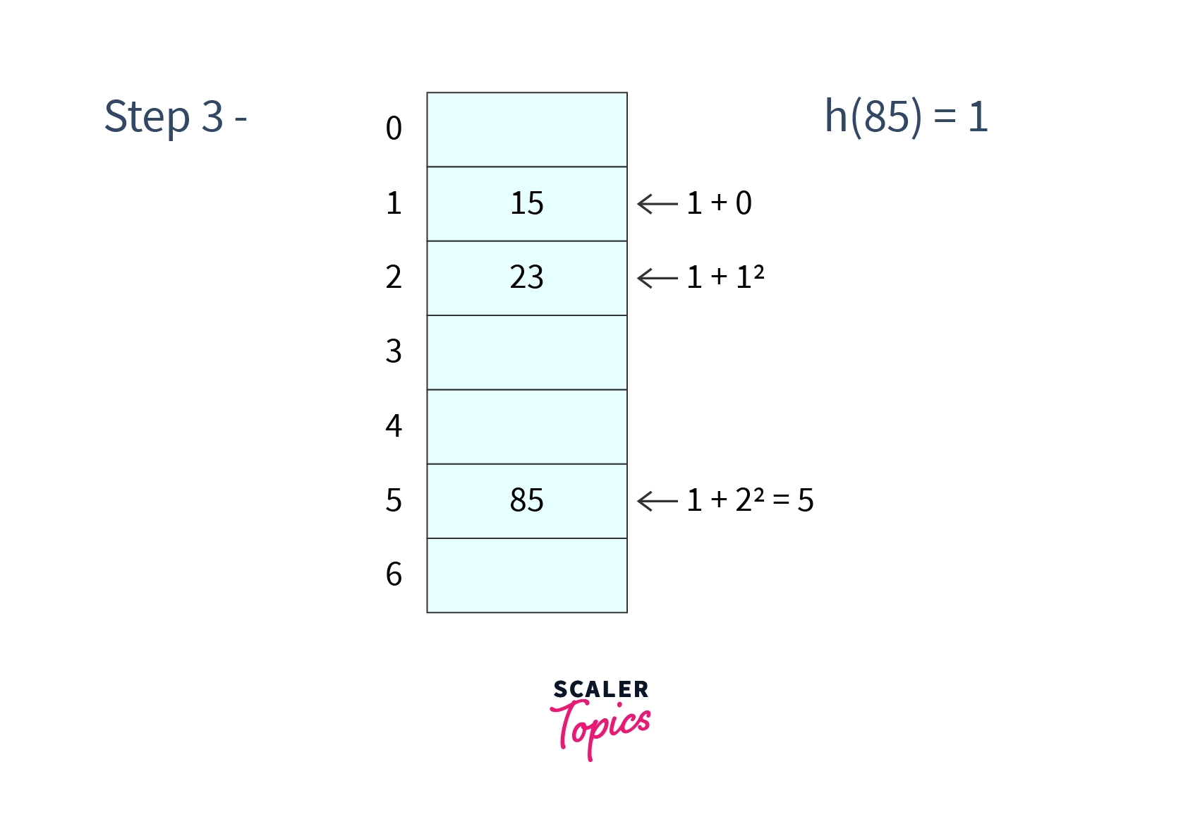
-
In our hash table cell 1 is already occupied so we will search for cell cell .
Again it is found occupied so we will search for cell cell . It is not occupied so we will place in cell .
After performing all these insertions in our hash table it will look like -
-
Step 4 - Search and delete We will go through the same steps as in inserting 85 and when we find 85 our search is successful and to delete it we will replace it with some other unique value a good choice is to replace it with .
Now as there is not much change in the approach of quadratic probing and linear probing. We are skipping algorithm and pseudocode of quadratic probing and directly jumping to its code.
Code of quadratic probing
- C/C++
- Java
Output -
Problem with Quadratic Probing
It can be observed that when the hash value for two keys, say and is the same then they will follow the same probe sequence because . Which leads to a milder form of clustering, called secondary clustering.
Another problem which can be more severe is, we are not sure if we can probe all the locations of our table. In other words, it can be said that there is no guarantee of finding an empty cell if the table is more than half-filled. The problem can be more severe when the size of the table is not a prime number.
Luckily :relieved: , to pose a solution to this problem, we have a theorem saying that -
- If the table size is prime and then all probes will be to a different location and an element can always be inserted in the hash table.
Turn Learning into Career Growth
Bonus Tip of Quadratic Probing
There are a lot of costly mathematical operations like and used in quadratic probing which can make it a little slow when dealing with huge input. To overcome this difficulty we can use some of our mathematical knowledge, by using this trick - Let, for any given , then it can be rewritten as , of course with taking modulus with table size wherever needed.
Double Hashing
Double hashing offers us one of the best techniques for hashing with open addressing. The permutation formed by double hashing is like a random permuatation therefore it almost eliminates the chances of cluster forming as it uses a secondary hash function as an offset to deal with collision condition.
The hash function that is used in double hashing is of the form -
A convenient and reasonable way to choose hash functions, and for a table of size, "" is like -
Where should be a prime number and can be slightly less than (say, ). The reason to add in is to avoid getting as , because if for any we get as then we will have .
By now, you might have got an idea about how you will do operations double hashing. So you can implement it like shown below - Operations in double hashing technique are -
- For inserting we search for the cells until we find an empty cell to insert . From here you can observe that if we don't get any collision at first (from the hash value of , we will not calculate because we can simply place at the index
- For searching we again search for the cells until we find a cell with value . If we find a cell that has never been occupied it means is not present in the hash table.
- For deletion, we repeat the search process if a cell is found with value we replace the value with a predefined unique value to denote that this cell has contained some value in past.
Example of double hashing
Table size = 7 = and Insert = and Search & Delete =
-
Step 1 - Create a table of size .
-
Step 2 - Insert and .
There is no collision at any point during inserting these three values so we will simply place these elements at their respective positions. After which, our hash table will look like -
-
Step 3 - Insert and
-
But at the cell at index 5 is already occupied, so we will check for next cell which will evaluate to . Cell at index 3 is not occupied so we will place 40 in cell 3.
-
But at the cell at index 4 is already occupied, so we will check for next cell which will evaluate to . Cell at index 0 is not occupied so we will place 74 in cell 0.
After which our hash table will look like -
-
-
Step 4 - Search and Delete
We will firstly search in cell 4 which does not contain so we will search for the next cell which may contain 74 which will evaluate to . We find in the cell at index 0 so our search is successful and now to delete it we replace its value with a very large number (say ).
After all the steps our hash table will look like -
Since the algorithm is not very different from the above two methods of hashing with open addressing we are directly going to code of Double Hashing -
Code of double hashing -
- C/C++
- Java
Output -
Analysis of Open Addressing
It is can be seen that, the cost of Insert, Search and Delete operations depends on how much the hash table is filled. More formally, we can say performance is related to load factor (). Time required to perform any operation increases as increases. With some mathematical proofs, we can say that it takes roughly time operate in the hash table if we are using open addressing.
Now we will look at the relative efficiency between the three collision resolution strategies that we have discussed.
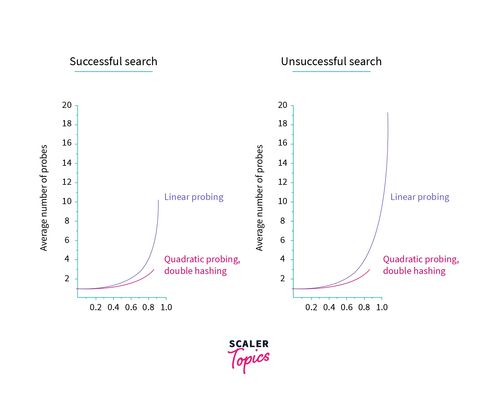
From the above image, we can see that performance of quadratic probing and double hashing is almost similar but Linear probing took a very large number of probes for an operation when the table is more than half-filled. The main difference between the above three strategies is that, linear probing provides the best cache performance but the clustering problem is very much evident in it. Double hashing exhibits poor cache performance but there is very less or no clustering problem. While quadratic probing lies between the two in both of the fields.
Advantages of open addressing -
- Open addressing provides better cache performance because all the data is stored in the same table only.
- It is easy to implement as no pointers are not involved.
- Different strategies to resolve collisions can be adopted as per the use case.
Practice Problems of Hashing with Open Addresssing
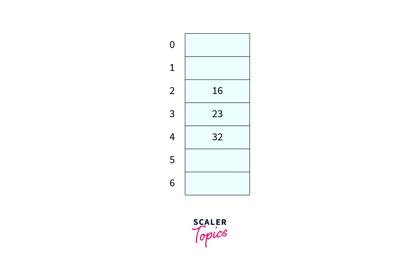
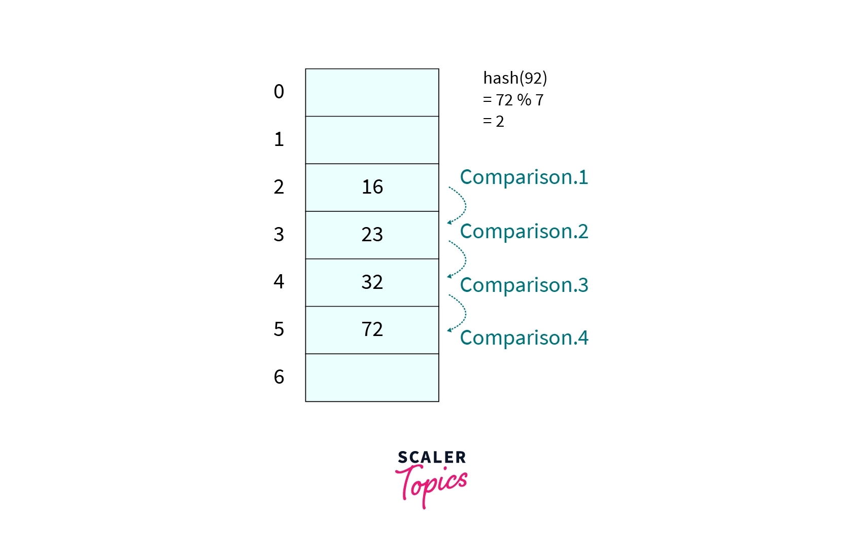
Given the hash table of size 7, already three keys are inserted as shown in the image. What will be the number of comparison required to insert in the hash table if the hash function is ?
Answer
Correct Answer - 4
Explanation -
KaTeX parse error: Expected 'EOF', got '%' at position 12: hash(72)=72%̲7=2 so we will begin our probe from 2nd index of the hash table and it will take 4 comparison to insert 72 in the hash table.
Image -
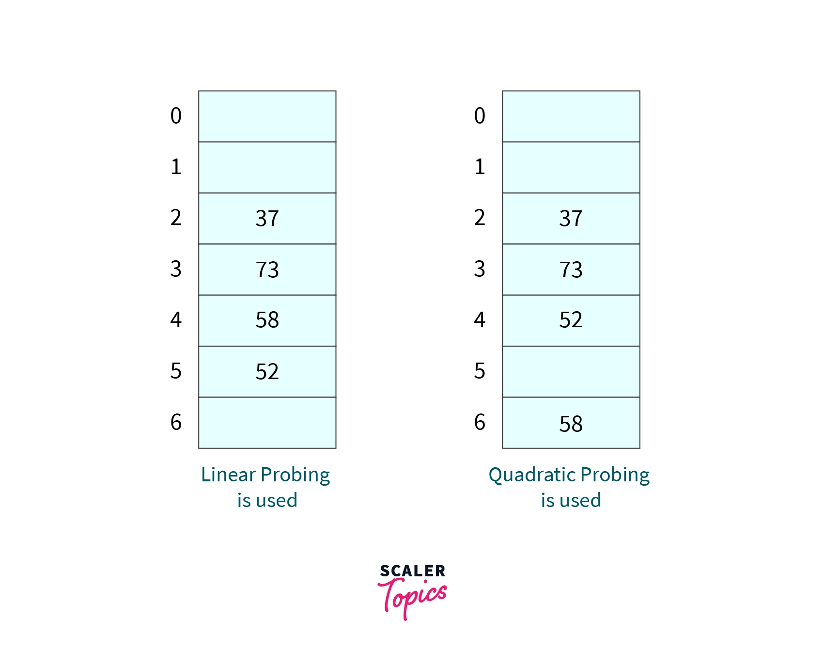
A hash function is defined by , If keys that are inserted into a hash table of size 7 are 37, 73, 58, and 52. Answer the following questions -
- What will be the position of 52 in the hash table, if the linear probing strategy is used to resolve the collision?
- What will be the position of 58 in the hash table, if the quadratic probing strategy is used to resolve the collision?
Answers
Position of 52 if linear probing is used is -
Position of 58 if quadratic probing is used is -
Explanation -
Below are the hash tables after performing the insertion operations. They are self-sufficient to explain the solutions.
Conclusion
- In this article, we have seen how we can use open addressing to resolve collisions during hashing process.
- Three collision resolution strategies have been discussed viz. Linear Probing, Quadratic Probing, and Double Hashing.
- Remember that, try to keep load factor () below and table size as a prime number unless it is unavoidable.
Code with Confidence! Enroll in Our Online Data Structures Courses and Master Efficient Algorithms.