Speech Recognition Architecture

Introduction

First, we will cover a brief introduction to speech recognition. When we say speech recognition, we’re talking about ASR or automatic speech recognition, in which for any continuous speech audio input, the corresponding output text should be generated. The architecture of the automatic speech recognition model consists of many components, which makes it difficult to build a robust automatic speech recognition system.

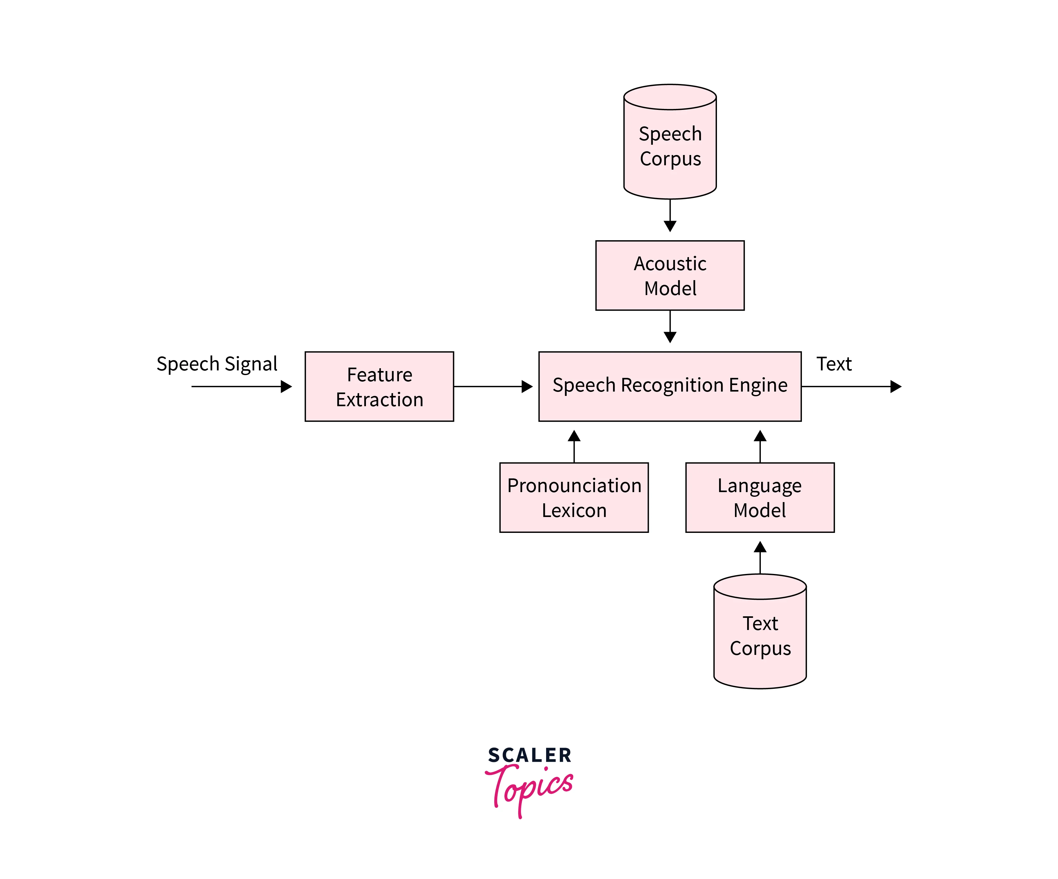
The above image describes the general architecture of Automatic Speech Recognition.

What Makes Speech Recognition Hard?

ASR is just like other machine learning problems, where the objective is to classify a sound wave into one of the basic units of speech, such as a word. The problem with human speech is that it contains a huge amount of variation in tone, pitch, and ascent that occurs while pronouncing a word.

There are several reasons for this variation, namely stress on the vocal cords, environmental conditions, microphone conditions, and many other reasons. To capture these variations in speech, machine learning algorithms such as Hidden Markov Model(HMM) with the Gaussian mixture model are used. In recent years Deep Neural Networks are also being used.

Challenges in Speech Recognition

There are a few challenges involved in developing speech recognition models

• Building a model of high accuracy
• language, accent, dialect coverage
• security and privacy
• cost and deployment

Models of High Accuracy

The accuracy of a speech recognition model needs to be high if it is to create any value for the business. However, achieving a high level of accuracy can be challenging. 73% of respondents claimed that accuracy was the biggest hindrance in adopting speech recognition tech.

There are certain factors to consider while evaluating models. These factors are usually responsible for not being able to achieve higher accuracies.

• Speech patterns and accents across the different regions of people, and people within those regions might have a different way of speaking, which makes training a model to recognize accents and speech patterns very difficult.
• when multiple speakers are present, they will frequently interrupt each other or speak at the same time, which can be a challenging task to transcribe for even the most experienced human transcribers.
• Additionally, ambient noise from music, talking, and even wind noise will affect the accuracy of transcription, as the computer uses sound bites to find out the word, and these other sounds can cause inaccuracies.
• These models will recognize words or phrases that are specifically trained to recognize. Before diving into the barriers to accuracy, it would be appropriate to mention that Word error rate (WER) is a commonly used metric to measure the accuracy & performance of a voice recognition system.

The Challenge of Language, Accent, and Dialect Coverage

Another significant challenge is enabling speech recognition to work with different languages, accents, and dialects. There are more than 7000 languages spoken in the world, with an uncountable number of accents and dialects. English alone has more than 160 dialects spoken all over the world.

The Challenge of Security and Privacy

A voice recording of someone is used as their biometric data, and due to that, many people are hesitant to share their voice samples. Most of us use smart devices such as google home, amazon Alexa, which collect voice data to improve the accuracy of their speech recognition model. Some people are unwilling to share this biometric information as this may help hackers to steal their data.

The Challenge of Cost and Deployment

Developing and maintaining speech recognition models are a costly and ongoing process. If the speech recognition model covers various languages, dialects, and accents, it needs a huge amount of training data and labeled data and huge computational resources.

Signal Analysis

Sound travels in waves that propagate through vibrations in the medium the wave is traveling in. No medium, no sound. Hence, sound doesn't travel in space. Below are the various methods to analyze speech signals:

• Fourier Transform
• Fast Fourier Transform
• Spectogram

Why Do We Use Fourier Transform for Signal Analysis?

Fourier transforms are used for sound wave analysis because they allow for the representation of a complex signal, such as a sound wave, as the sum of simpler sinusoidal signals. This makes it possible to understand and analyze the individual frequency components that make up the overall sound wave, which can be useful for tasks such as filtering or compression. Additionally, the Fourier transform can be used to analyze the frequency content of a sound wave in the time domain, which can be useful for tasks such as identifying the presence of certain frequencies or determining the pitch of a sound.

Fourier Transfrom

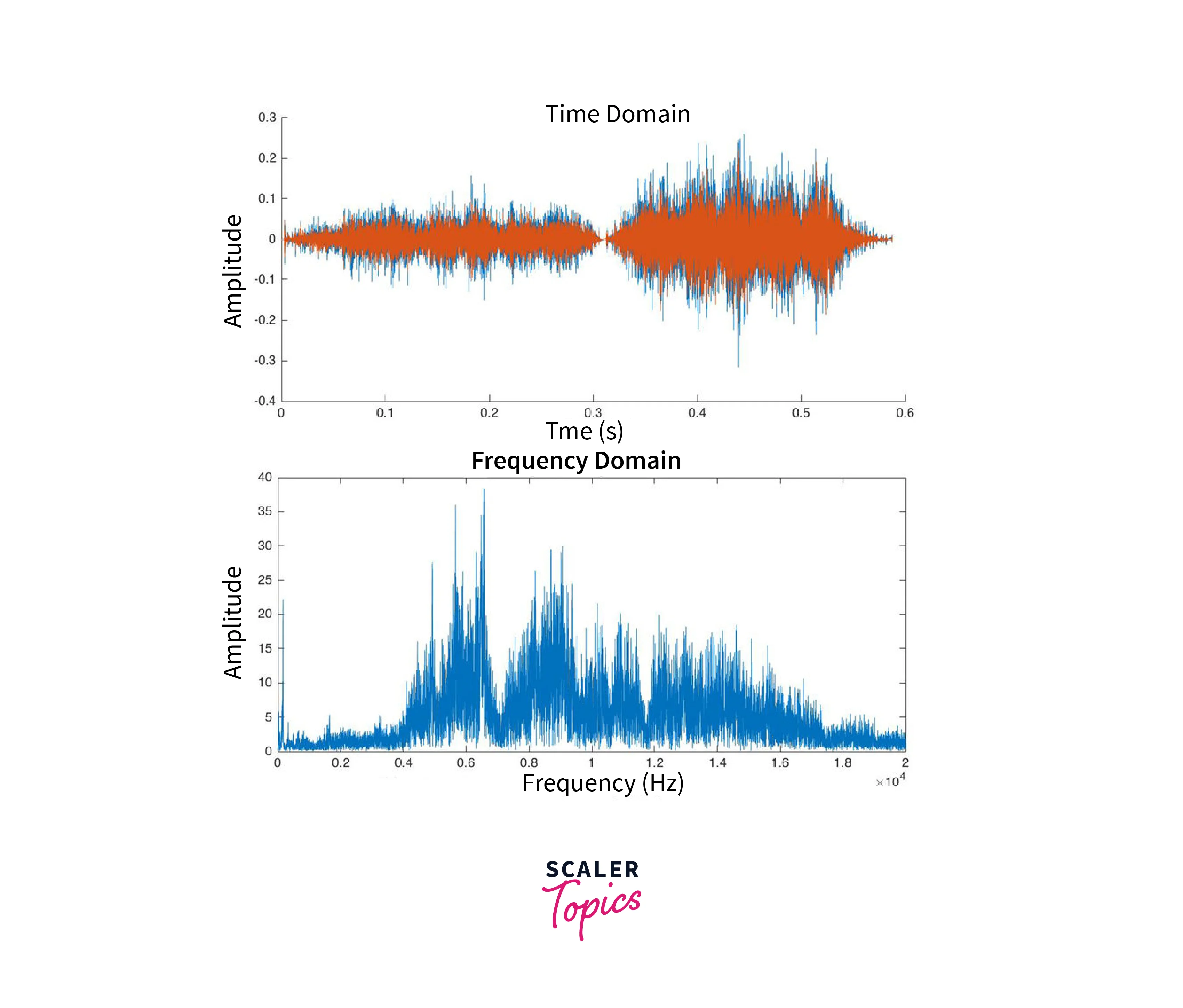
An audio signal is a complex signal composed of multiple single frequencies of sound waves, which travel together as a disturbance in a medium. When sound is recorded, we only capture the resultant amplitude of those multiple waves.

Fourier transform is a mathematical concept that can decompose a signal into its constituent frequencies. It gives not only the frequencies present in the signal but also the magnitude of each frequency present in the signal

Fast Fourier Transfrom

It is a mathematical algorithm that calculates the Discrete Fourier transform of a given sequence. The only difference between Fourier Transform(FT) and Fast Fourier Transform (FFT) is that FT considers a continuous signal while FFT considers a discrete signal as an input.

DFT converts a sequence (discrete signal) into its frequency constituents just like FT does for a continuous signal. We have a sequence of amplitudes that were sampled from a continuous audio signal. DFT or FFT algorithm can convert this time-domain discrete signal into a frequency-domain.

Spectrogram

Visual representation of frequencies of a given signal with time is called Spectrogram

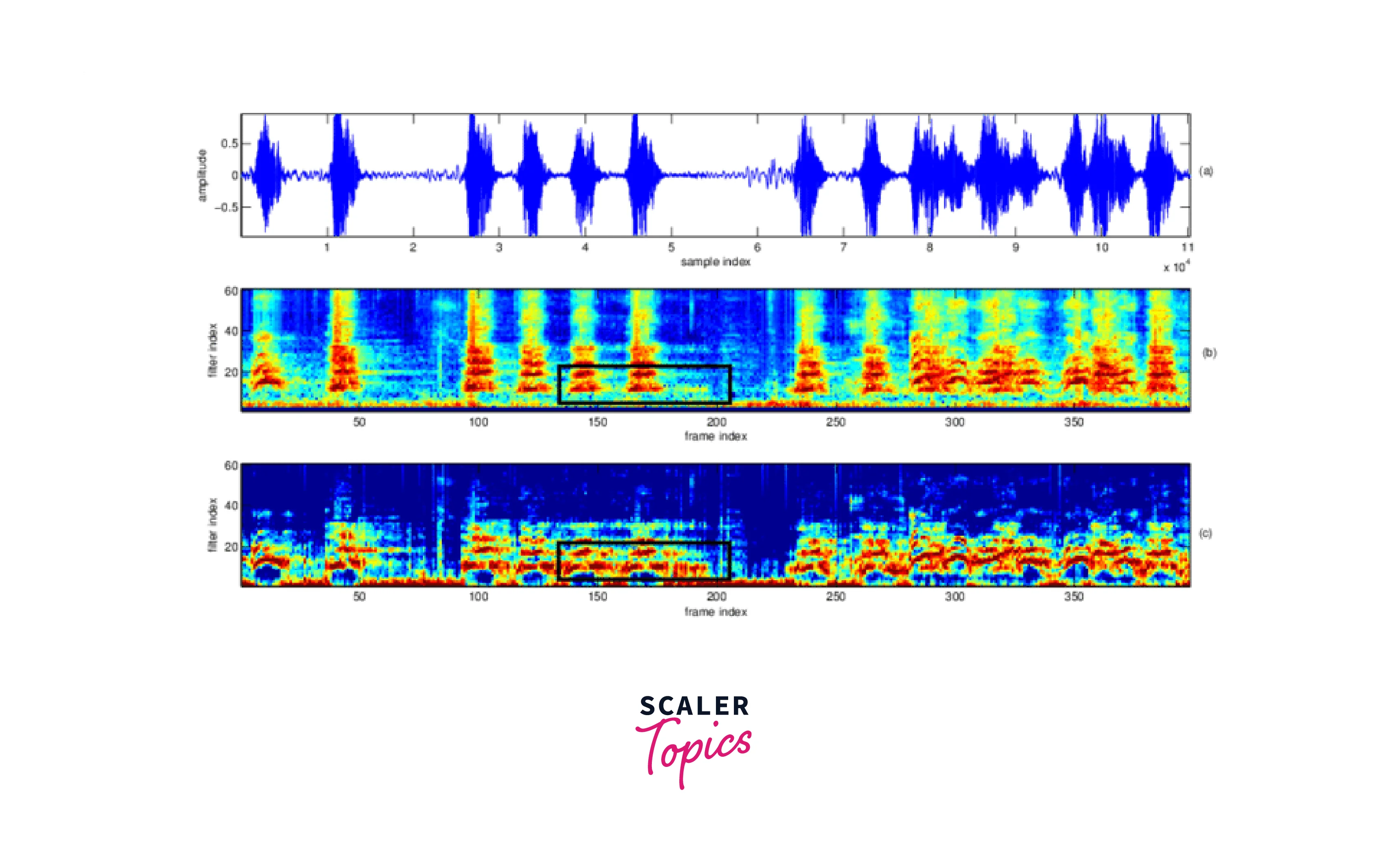
Spectrogram representation plot — one axis represents the time, the second axis represents frequencies, and the colors represent the magnitude (amplitude) of the observed frequency at a particular time.

Bright colors represent strong frequencies. Similar to the earlier FFT plot, smaller frequencies ranging from (0–1kHz) are strong(bright).

HMMs in Speech Recognition

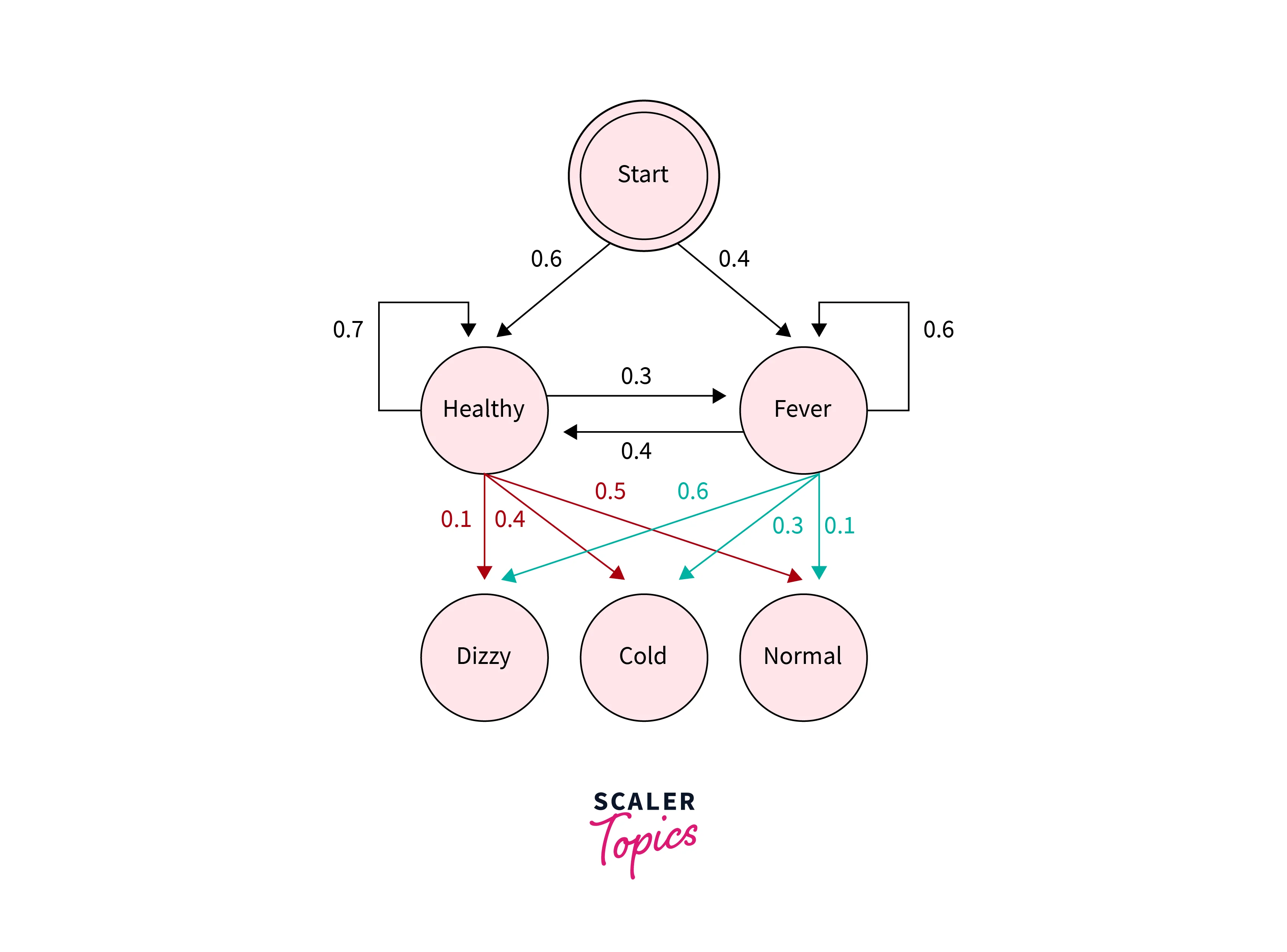
The hidden Markov model works based on the Markov process, A Markov chain is a mathematical model used in speech recognition to model the probability of a sequence of words or sounds. It is based on the assumption that the probability of a certain word or sound depends only on the preceding words or sounds in the sequence and not on the preceding words or sounds before that.

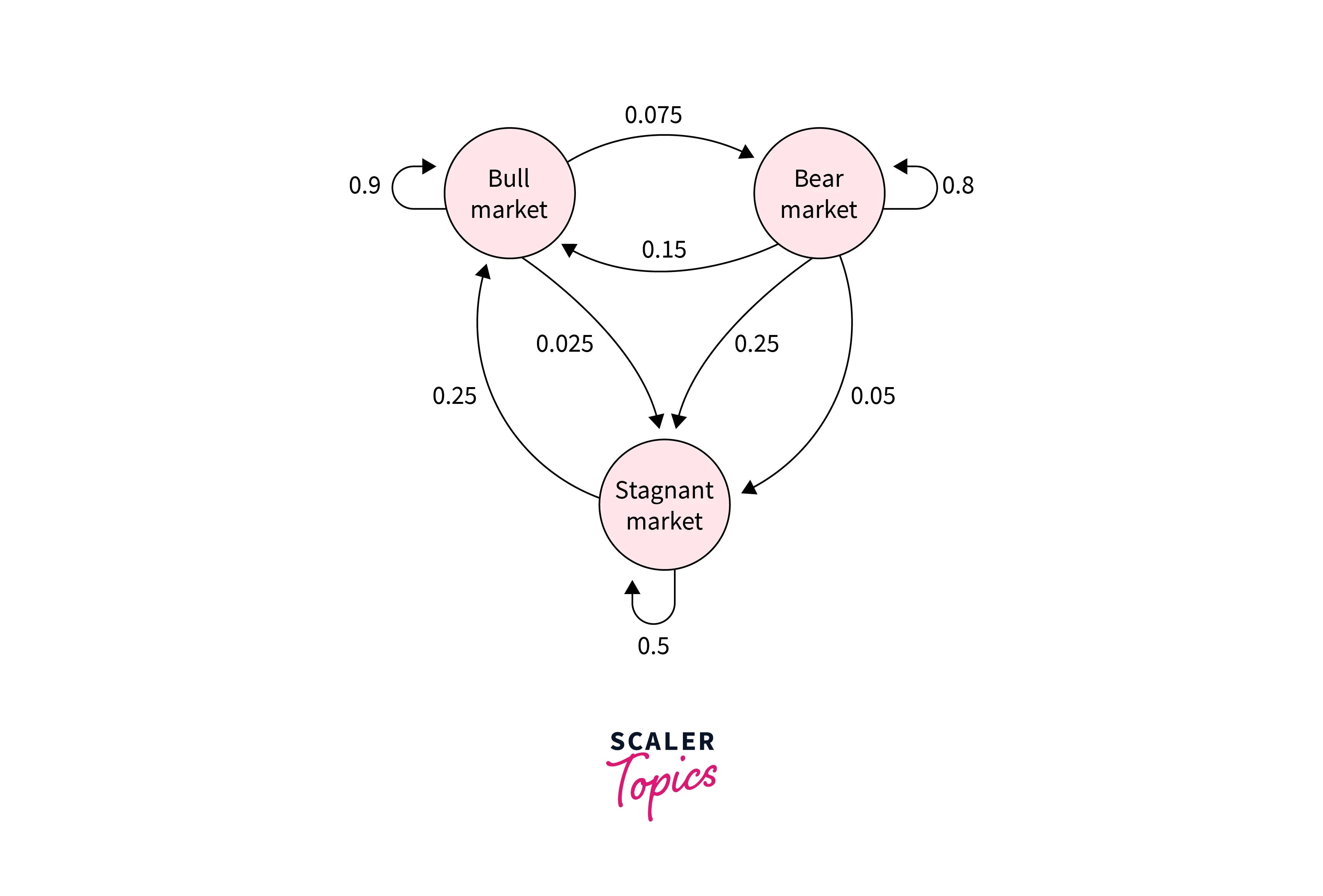
A first-order Markov chain assumes that the next state depends on the current state only. It will not depend on any other previous states for predicting the next state.

In many ML systems, not all states are observable, and we call them hidden states or internal states.

Suppose we have a dataset of speech samples that contains the words "hello" and "world" spoken by different speakers. We want to train an HMM-based ASR system to recognize these two words.

First, we need to segment the speech samples into a sequence of phonemes, which are the smallest unit of sound that can distinguish one word from another. For example, the word "hello" can be segmented into the phonemes /h/ /ɛ/ /l/ /o/.

Next, we create an HMM for each word, with states corresponding to the phonemes and the probability distributions over the observations. For example, the HMM for the word "hello" would have five states, one for each phoneme, and the probability distributions for the observations in each state would be estimated from the dataset.

Once the HMMs are trained, we can use them to recognize speech. Given a new speech sample, we compute the likelihood of the sample given each HMM, and the HMM with the highest likelihood is considered the recognized word.

In this example, the observation sequence is transformed into a sequence of feature vectors, which are a set of acoustic-prosodic features of the speech signal, such as pitch, energy, and spectral content. The HMM is trained using these feature vectors.

The probability of observing an observable, given an internal state, is called the emission probability. The probability of transiting from one internal state to another is called the transition probability.

Viterbi Algorithm

The main use of this algorithm is to make inferences based on a trained model and some observed data.

The algorithm starts by initializing a matrix called the Viterbi matrix, which is used to store the maximum likelihood of each state at each time step. The algorithm then iterates over the observations, updating the Viterbi matrix at each time step.

At each time step, the algorithm considers all possible states and computes the likelihood of the current observation given each state. It also takes into account the maximum likelihood of each state at the previous time step, as well as the transition probabilities between states.

The algorithm then selects the state that maximizes the likelihood at each time step and records the path in a matrix called the back pointer matrix. Once the final observation is reached, the algorithm selects the final state that maximizes the likelihood, and the path through the states that leads to this final state is the most likely sequence of states given the observations.

N-Gram Language Model

An N-Gram language model is a sequence of N Tokens (Words). Tokens are nothing but the neighboring sequence of items in a document.

In an N-gram model, the N refers to the number of items in a sequence. An N-gram is a contiguous sequence of N items from a given sample of text or speech. It can go from 1,2,3...to n, and each has a name associated with it as follows:

1 -------- Unigram --- [“I”, ”Love”,” Bengaluru”,“so”,"much"] 2 -------- Bigram --- [“I Love”,” Love Bengaluru”, ”Bengaluru so”," so much"] 3 -------- Trigram --- [“I Love Bengaluru”, “Bengaluru so much”]

From the table above, it’s clear that unigram means taking only one word at a time, bigram means taking two words at a time, and trigram means taking three words at a time.

How N-gram Language Models Work?

An N-gram language Model predicts the probability of a given N-gram within any sequence of words in the given language.

An N-gram language model estimates the probability of a word given the precedingN-1words based on the frequency of N-grams seen in the training data. This allows the model to predict the probability of a word, given a history of previous words, where the history contains N-1 words.

Limitations of the N-gram Model

• Higher the value of N, the better the model will learn, but it needs a lot of computation power, i.e., a large amount of RAM and GPU

• Data Sparsity: N-gram models rely on the frequency of N-grams seen in the training data. However, if a certain N-gram is not present in the training data, the model will assign a zero probability to it, even if it's a valid sequence. This is known as the data sparsity problem.

• Curse of Dimensionality: N-gram models increase in complexity as the value of N increases, which can lead to a large number of parameters that need to be estimated. This can cause the model to overfit the training data and perform poorly on new data.

• Lack of context: N-gram models only take into account the preceding N-1 words, which may not be enough context to make an accurate prediction. This can be especially problematic for words that have multiple meanings depending on the context.

• Lack of generalization: N-gram models are based on the frequency of N-grams in the training data. However, this may not generalize well to new data that may have different word frequencies.

Speaker Diarization (SD)

Speaker diarization , also known as "who spoke when," is the process of automatically determining who spoke when in a given audio or video recording. It is a form of speaker segmentation, and it aims to partition an audio or video recording into segments corresponding to individual speakers.

There are several techniques used in speaker diarization, such as clustering, classification, and decoding. Clustering techniques group similar speech segments together based on acoustic features, such as pitch, energy, and spectral content. Classification techniques use machine learning to classify speech segments as belonging to a particular speaker based on acoustic features. Decoding techniques use a probabilistic model, such as a Hidden Markov Model (HMM) or a Deep Neural Network (DNN), to infer the most likely speaker at each time step.

Speaker diarization is a challenging task due to the dynamic nature of speech, such as overlapping speech, speaker variability, and background noise. It has a wide range of applications, such as meeting summarization, media monitoring, and forensic analysis.

In recent years, deep learning techniques have been used to improve the performance of speaker diarization systems, such as using deep neural networks for feature extraction or using end-to-end neural models for speaker diarization.