Backoff in NLP

Introduction

First, we will briefly understand what language models are, what N-gram models are, what are the issues that arise with estimating probability distributions and, in turn, the parameters of these models, and then see how smoothing methods like backoff techniques can help solve these problems.

Language models

One of the underlying ideas behind language models is the simple idea that some word sequences are more frequent than others, which led to the development of language models for text and also gave rise to mainstream NLP research.

• Statistical Language Models (SLMs), in particular, are based on n-grams and are now widely used in most of the NLP fields.
• Statistical Language Models have the power to represent some crucial aspects of language and also are quick and easy to implement, and do not require the labor-intensive development of NLP resources such as dictionaries or grammar, making them ideal for research in relatively resource-poor languages also.
• N-gram language models: Statistical language models can be viewed as a probability distribution over a set of possible sentences representing how often each sentence occurs in the modeled language.
  • The most widely-used SLMs are based on n-grams in which the probability of a given word in a sentence is determined by the n-1 previous words, which is also the recent history.
  • SLM computes probabilities based on the maximum likelihood (ML) estimates in the simplest form with some allowance for unseen instances.
  • In a trigram model, for example, the maximum likelihood conditional probability of a word wi given its two predecessors wi-2 and wi-1 is defined as the counting (c) of occurrences of the trigram divided by the number of occurrences of its bigram constituent.

Now, let us see what issues arise when estimating parameters and computing probabilities in these language models.

Issues with probability estimation in LM

When dealing with probability distributions to be estimated for language models, we come across scenarios related to determining the probability or likelihood estimate of a sequence of words (like a sentence) occurring together when one or more words individually (unigram) or N-grams such as bigramKaTeX parse error: Expected 'EOF', got '−' at position 7: (wi/wi−̲1) or trigramKaTeX parse error: Expected 'EOF', got '−' at position 7: (wi/wi−̲1wi−2) in the given set have never occurred in the past.

• Even if one n-gram is unseen in the sentence, the probability of the whole sentence becomes zero.
• Hence the probability of a test document given some class can be zero even if a single word in that document is unseen
• One way to avoid this is to allot some probability mass by reserving for the unseen words.
• Smoothing techniques are touted as solutions to tackle this major problem in building language models.
• Example of unseen word estimation using MLE: If we take the example of probability estimation using MLE, for the P(the | burnish). If the bigram "burnish the" doesn't appear in our training corpus, then P(the| burnish) = 0.
  • But we know that no word sequence should have 0 probability as that can’t be intuitively right.
  • Furthermore, MLE also produces poor estimates when the counts are non-zero but still small.
  • Hence the need for better estimators than MLE for rare events, which is solved by somewhat decreasing the probability of previously seen events so that there is a little bit of probability mass left over for previously unseen events.

What is Backoff?

The general idea of backoff is that it always helps to use lesser context to generalize for contexts that the model doesn’t know enough about.

• For example,we can use trigram probabilities if there is sufficient evidence, else we can use bigram or unigram probabilities.
• It is the concept where sentences are generated in small steps which can be recombined in other ways.
• If we have no examples of a particular trigram Wn-2, Wn-1, Wn, to compute $P(Wn|Wn-1, Wn-2)$, we can estimate its probability by using the bigram probability $P(Wn|Wn-1)$.

Why Do We Need Backoff in NLP?

We need techniques like smoothing (and backoff is a subset of smoothing techniques) to tackle the problems of sparsity and improve the generalization power of NLP models.

Issues of Sparsity in NLP

• Language models use huge amounts of parameters on data to build the NLP models, and sparsity becomes an issue, and incorporating proper smoothing techniques into the models usually leads to more accuracy than the original models.
• Data sparsity is another issue with language models, statistical modeling, and also NLP techniques in general, and smoothing can help with the performance issue.
• Sometimes, we come across the extreme case where there is so much training data, and even though all parameters can be accurately trained without smoothing, even in such cases, it is almost always usual to expand the model such as by moving to a higher n-gram model to achieve improved performance and smoothing can help with such cases too.

, For example,, in several million words of English text, more than 50% of the trigrams occur only once, and 80% of the trigrams occur less than five times.

Issues with Model Generalization in NLP

Language models, in general, use a huge amount of data for training, and the output of these models is dependent on the N-grams appearing in the training corpus. The models work well only if the training corpus is similar to the testing dataset; this is the risk of overfitting to the training set.

• As with any machine learning method, we would like results that are generalizable to new information.
• One of the other harder problems with language models and, in general, NLP is how we deal with words that do not even appear in training but are in the test data.

Thus, no matter how much data one has or how many parameters are there in the model, smoothing can almost always help performance for a relatively small effort.

Concept of Combining Estimators in NLP

• Typical probability estimation techniques like maximum likelihood estimation don't work when dealing with cases of unknown events where sparsity leads to poor performance.
  • We can choose to estimate the parameters with different smoothing estimation techniques like Laplace smoothing or good Turing discounting.
  • Smoothing methods provide the same estimate for all unseen or rare n-grams with the same prefix making use only of the raw frequency of the n-gram.
• One other method is to combine a complex model with simpler models with techniques like linear interpolation or modified Kneser-Ney smoothing or back-off techniques.
• Backoff techniques utilize the additional source of knowledge based on the n-gram hierarchy.
  • We can estimate the probability of those particular trigrams where there are no examples by using the bigram probability, and further, if there are no examples of the bigram to compute $P(Wn|Wn-1)$, then we can use the unigram probability $P(Wn)$ as a step ahead.
  • Hence suitably combining various models of different orders is the secret to success for n-gram models.
  • The n-gram models at level n can be combined with the models for the shorter unigrams to (n-1)-grams.

Good-Turing Discounting

Good Turing discounting is one of the useful techniques in smoothing to improve the model accuracy by taking into account additional information about the data distribution.

The basic idea behind good Turing smoothing is to use the total frequency of events that occur only once to estimate how much mass to shift to unseen events.

• Good-Turing estimator (GT) developed by Gale & Sampson in 1995 assumes the probability mass of unseen events to be n1 / N, where N is the total of instances observed in the training data and n1 is the number of instances observed only once.
• Reassign the probability mass of all events that occur k times in the training data to all events that occur k–1 times.
• Re-estimates the amount of probability mass to assign to N-grams with zero or low counts by looking at the number of N-grams with higher counts.

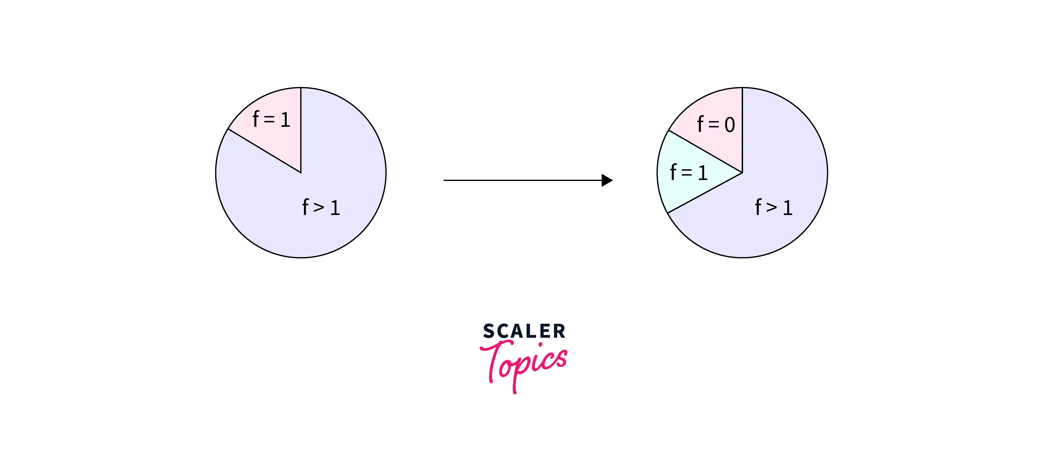
• As you can see in the above illustration, we take the probability of N-grams with lower values and give it to ones with zero.
• It is the norm to treat Ngrams with low counts, for example, with very small counts of one, as if the count was 0 in all the discounting methods.
• Advantages of Good Turing Discounting: Good Turing discounting Works very well in practice.
  • Usually, the excellent Turing discounted estimate is used only for unreliable counts, for example, for counts less than 5.
• Disadvantages with Good Turing Discounting: There are two main problems with good Turing discounting.
  • The reassignment may change the probability of the most frequent event, and also, we generally don’t observe events for every k.
  • Both of these problems can be solved by a variant of good Turing called Simple Good-Turing Discounting.

N-gram Backoff

Concept of N-gram Backoff

The central idea in n-gram backoff is to approximate the probability of an unobserved N-gram using more frequently occurring lower order N-grams.

• If we are trying to compute $P\left(w_n \mid w_{n-2} w_{n-1}\right)$, but we have no examples of a particular trigram $w_{n-2} w_{n-1} w_{n}$, we can instead estimate its probability by using the bigram probability $P\left(w_n \mid w_{n-1}\right)$.
• Similarly, if we don’t have counts to compute $P\left(w_n \mid w_{n-1}\right)$, we can look to the unigram $P(w_n)$. Hence if an N-gram count is zero, we approximate its probability using a lower order N-gram.

General Formula for Backoff

\begin{aligned} &P\left(w_n \mid w_{n-1}, w_{n-2}\right) \ &=P^*\left(w_n \mid w_{n-1}, w_{n-2}\right), \text { if } C\left(w_{n-2}, w_{n-1}, w_n\right)>0 \ &=\alpha\left(w_{n-1}, w_{n-2}\right) P\left(w_n \mid w_{n-1}\right), \text { otherwise } \end{aligned}

• Where P* is discounted probability (non-MLE probability) to save some probability mass for lower order n-grams
• α(wn-1,wn-2) is to ensure that probability mass from all bigrams sums up exactly to the amount saved by discounting in trigrams.
• The scaling factor is chosen to make the conditional distribution sum to one.

Example for N-gram Backoff

• If we consider the example i spent xxx, and let's say the trigram i spent in occurs only once, the probability of word / i, spent is 1 if the word is in and 0 for all other words.
• But the bigram spent three may occur many times when we look at bigram tokens beginning with spent, so we these instead to compute the probability.

Main Advantage of N-gram backoff: Extremely popular for N-gram modeling in speech recognition because we can control complexity as well as generalization.

Discounted Backoff

Need for Discounting in Backoff

• While modeling probabilities with backoff, higher-order n-grams are explicitly discounted and the n-gram which has zero probability is replaced with a lower-order n-gram in backoff.
  • This will add probability mass and the total probability assigned to all possible strings by the language model would be greater than 1!
  • Hence the need to modify the discounted MLE probabilities also.
• So, in addition to the explicit discount factor (from higher grams to lower ones), we develop a function to distribute the additional probability mass to the lower order n-grams, which is done by the Discounted Backoff.

Katz Backoff

Katz backoff is another way to solve the issue of a zero-probability word sequence in typical sparse train datasets where the corpus is limited and finite in size.

• We rely on a discounted probability P∗ if we’ve seen the n-gram before if we have non-zero counts, and otherwise, we recursively back off to the Katz probability for the shorter-history (N-1)-gram.
• Utilising the Katz backoff will help in assigning meaningful probabilities to acceptable word sequences in the language considered, which are missing in the dataset.
• The concept of discounting in Katz backoff involves subtracting a fixed discount D from each non-zero count for the n-grams (or entities) and then redistributing this probability mass to N-grams with zero counts.
• Discounting can also be seen as a kind of additional smoothing step in the algorithm which introduces a discount factor which is the ratio of the discounted counts to the original count
• Hence discounting is the way of lowering each non-zero count c to c* (c > c*) according to the smoothing algorithm.

Stupid Backoff

There's too much information to use interpolation effectively when we are dealing with web-scale applications, and therefore we need a different backoff technique.

• In Stupid Backoff, we use the trigram if we have enough data points to make it seem credible; otherwise, if we don't have enough of a trigram count, we back off and use the bigram, and if there still isn't enough of a bigram count, we use the unigram probability.
• Instead of the discounting step in the smoothing procedure, we can use the relative frequencies of the words alone.
• The method is named stupid because the initial thought when the method was proposed was that such a simple scheme can’t be possibly good.
• Eventually, the method turned out to be as good as the state-of-the-art Kneser Ney smoothing.

Equations for Stupid Backoff

\begin{aligned} &S\left(w_n \mid w_{n-1}, w_{n-2}\right)\ &=\frac{C\left(w_{n-2}, w_{n-1}, w_n\right)}{C\left(w_{n-2}, w_{n-1}\right)} \text {, if } C\left(w_{n-2}, w_{n-1}, w_n\right)>0\ &=\alpha S\left(w_n \mid w_{n-1}\right) \text {, otherwise }\ &S\left(w_n\right)=\frac{C\left(w_n\right)}{\text { Size of training corpus }} \end{aligned} The symbol S is used instead of the probability symbol P as these are not probabilities but scores.

Advantages of Stupid backoff

• Inexpensive yet accurate calculations with large training sets: Stupid Backoff is inexpensive to calculate in a distributed environment while approaching the quality of Kneser-Ney smoothing for large amounts of data.
• The lack of normalization also does not affect the functioning of the language model as smoothing based on stupid backoff depends on relative rather than absolute feature-function values.
• Inexpensive to calculate for web-scale n-grams.

Deleted Interpolation

Interpolation is another smoothing technique to combine knowledge from multiple types of N-gram* into the computation of the probabilities. Deleted interpolation is similar to backoff, where for computing trigram probability, we use the bigram and unigram information of focus words.

• The main difference with backoff is that if we have non-zero trigram counts, we rely on these trigram counts completely instead of interpolating with bigram and trigram counts.

• We can also say that we are linearly interpolating a bigram and a unigram model when combining bigrams and unigrams with trigrams. We can generalize this to interpolating an N-gram model using an (N-1)-gram model.

  • We need to note that this leads to a recursive procedure if the lower order N-gram probability also doesn't exist & hence if necessary, everything can be estimated in terms of a unigram model.

• A scaling factor is also used to make sure that the conditional distribution will sum to one.

  • An N-gram-specific weight is used, and it would lead to far too many parameters to estimate. In such cases, we need to cluster multiple such weights like with word classes suitably, or in extreme cases. We can also use a single weight if clustering doesn't work.

• Equation for simple linear interpolation: $\begin{aligned} \hat{P}\left(w_n \mid w_{n-2} w_{n-1}\right)=& \lambda_1 P\left(w_n\right) \\ &+\lambda_2 P\left(w_n \mid w_{n-1}\right) \\ &+\lambda_3 P\left(w_n \mid w_{n-2} w_{n-1}\right) \end{aligned}$

  • One constraint is that the λs must sum to 1.

• Concept of conditional interpolation λ: This is a slightly sophisticated version of linear interpolation where each λ weight is computed by conditioning on the context.

  • This way, if we have particularly accurate counts for a particular bigram, we assume that the counts of the trigrams based on this bigram will be more trustworthy.
  • So we can make the λs for those trigrams higher and thus give that trigram more weight in the interpolation.

• Finding values for λ: Both the simple interpolation and conditional interpolation λs are learned from a held-out corpus.

  • We choose the λ values that maximize the likelihood of the given held-out corpus.
  • We fix the n-gram probabilities and then search for the λ values that—when plugged into the overall equation, give us the highest probability of the held-out set.
  • We can also use the expectation maximization (EM) algorithm, which is an iterative learning algorithm that converges on locally optimal λs.

Comparison of Different Smoothing Techniques

• The relative performance of smoothing techniques can vary based on training set size, n-gram order, and also the quality of the training corpus.
• Backoff vs. Interpolation: Backoff is superior on large datasets because it is superior on high counts, while interpolation is superior on low counts.
  • Interpolation works well in scenarios with low counts as lower order distributions provide valuable information about the correct amount to discount, and thus interpolation is superior for such situations.
  • Katz backoff smoothing performs well on n-grams with large counts.
  • Kneser Ney smoothing is also one of the best for small counts.
• Algorithms that perform well on low counts perform well overall when low counts form a larger fraction of the total entropy in small datasets.
• Backoff, in general, performs better on bigram models than on trigram models as bigram models contain higher counts than trigram models on the same size data.