LSA – Latent Semantic Allocation

Introduction

LSA is primarily used for concept searching and automated document categorization. LSA tries to mimic humans way of word sorting and document categorization.

LSA is a popular dimensionality reduction technique that follows the same method as Singular Value Decomposition. LSA ultimately reformulates text data in terms of latent (i.e. hidden) features, where the number of these features should be less than the number of documents, and the number of terms in the data.

LSA can use a document-term (or document-word) matrix which describes the occurrences of terms in documents; it is a sparse matrix whose rows correspond to documents and whose columns correspond to terms.

After the construction of the occurrence matrix, LSA finds a low-rank approximation to the document-term matrix using SVD to reveal patterns in the relationships between the terms & concepts and documents & concepts which are contained in an unstructured collection of text.

That's a lot of technical jargon, let's try to understand LSA intuitively and get comfortable with the principles of LSA then we'll deep dive into its maths and code implementation.

The Intuition Behind LSA

In very simple words - If you have an M number of documents, and if you do the categorization manually you might come up with a k number of topics in which you can categorize these documents.

LSA also tries to come up with something close to k topics algorithmically. Even though identifying k topics by humans may not be accurate, the same goes for the LSA algorithm. The final decision will always be a judgemental call on whether these k topics/categories can accurately classify the documents, depending on the usecase as well.

Let's have a look at how raw data and data-term matrix looks like from sample documents belonging to several categories such as Data Science, Religion, Scientific Fiction Movies, etc (M documents).

Doc 1: Data science is a concept to unify statistics, data analytics, informatics, and their related methods to understand and analyze actual phenomena with data

Doc 2: Religious practices may include rituals, sermons, commemoration, sacrifices, festivals, feasts, trances, initiations, funerary services, matrimonial services, meditation, prayer, music, art, dance, public service, or other aspects of human culture

Doc 3: Science fiction is a film genre that uses speculative, fictional science-based depictions of phenomena that are not fully accepted by mainstream science, such as extraterrestrial lifeforms, spacecraft, robots, cyborgs, interstellar travel, time travel, or other technologies

Doc 4

Doc 5

Doc 6 . . . Doc M

Here we already know that the doc1 is from data science, doc2 is from religion and doc3 is from a sci-fi film

The sample of the document-term matrix is shown in the image below :

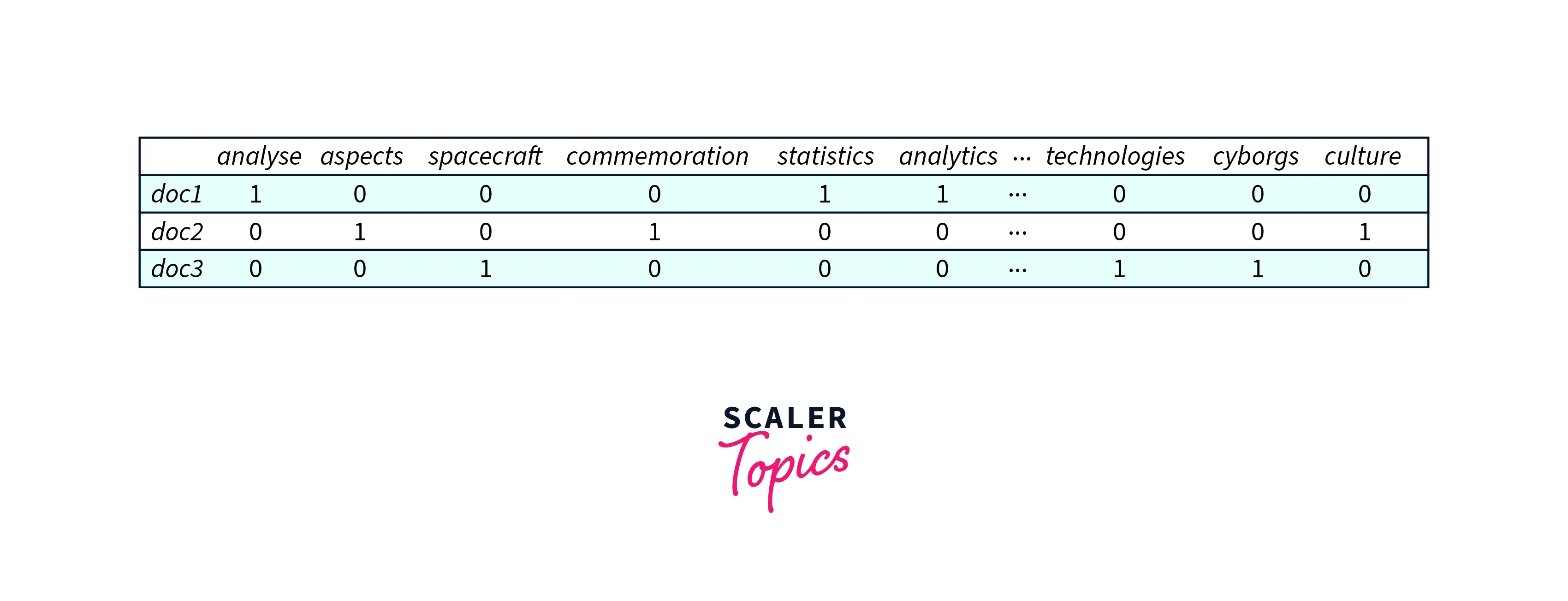
This table represents the word/term frequency in the document.

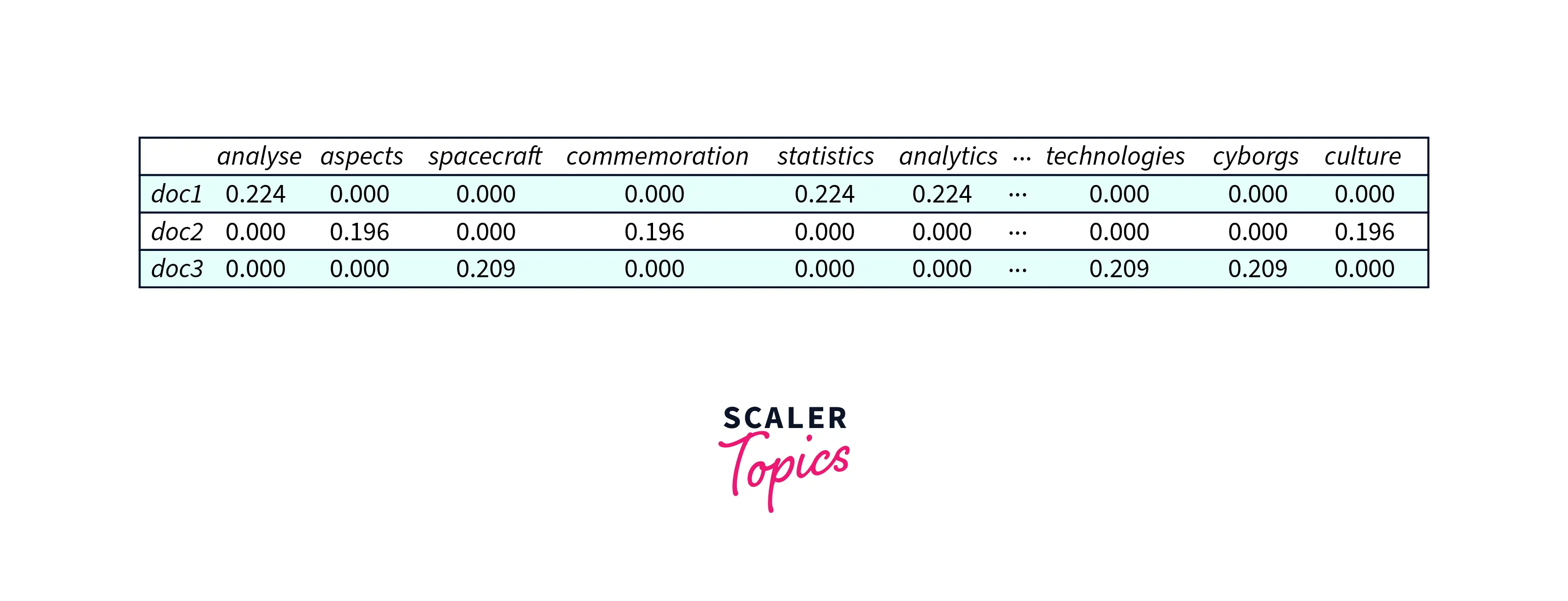
But we will use the standardized version of this table for LSA implementation. The Standardisation is done using TF-IDF vectorization.

Below is the standard version of this table :

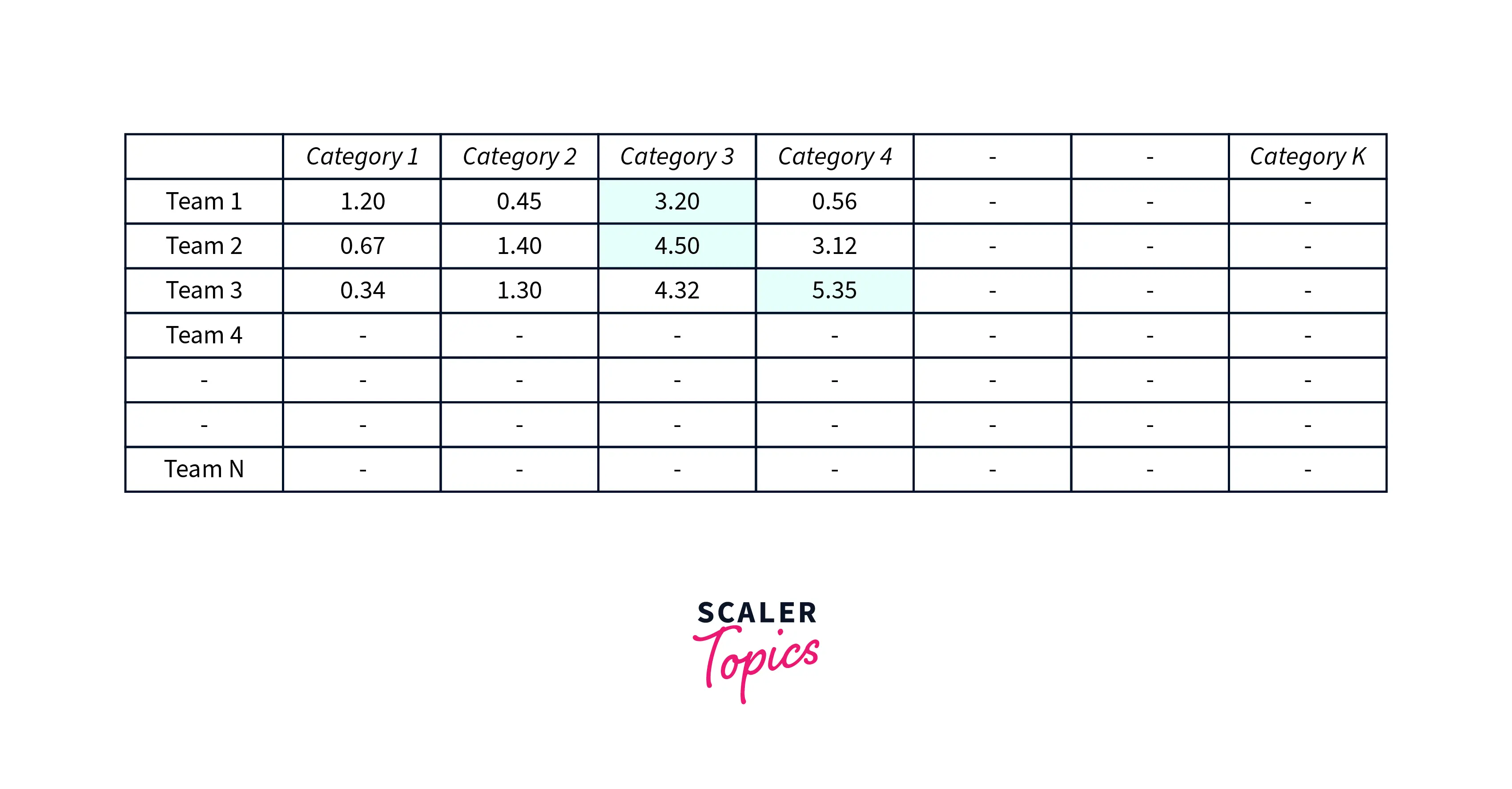
The final data-term matrix could look something like this:

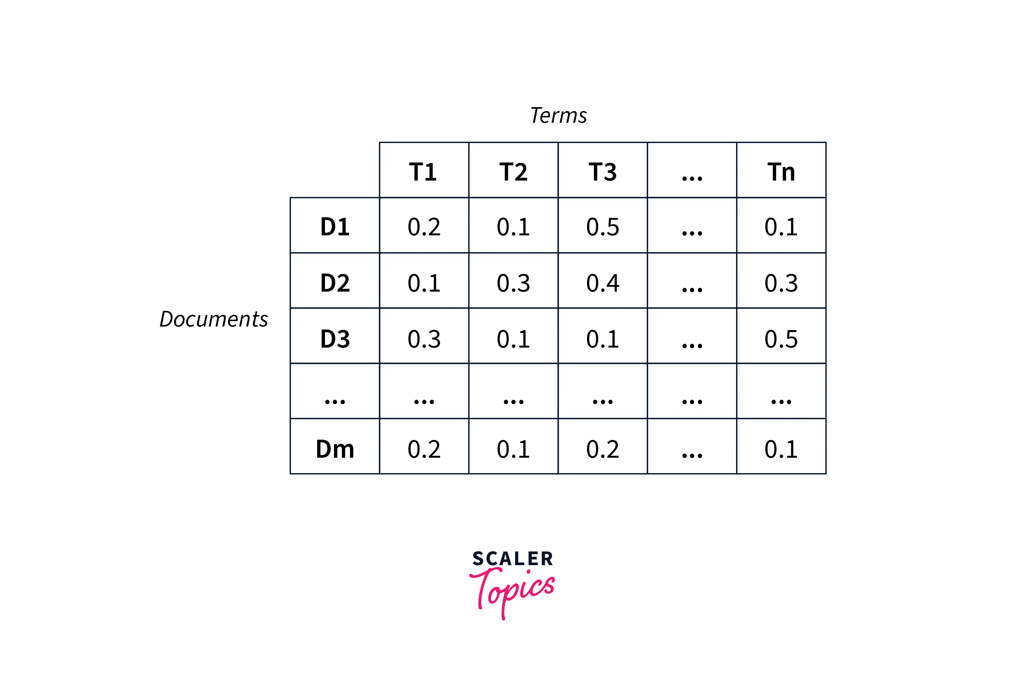
Here, In the cells, we would have different numbers that indicated how strongly that document belongs to the particular topic.

1. A document could strongly belong to a certain category

• This will be represented in a matrix called the document-category matrix (U) also called the document topic matrix

• Higher cell value indicates that this document is more explained by this category

• for our sample documents this matrix could look like this:

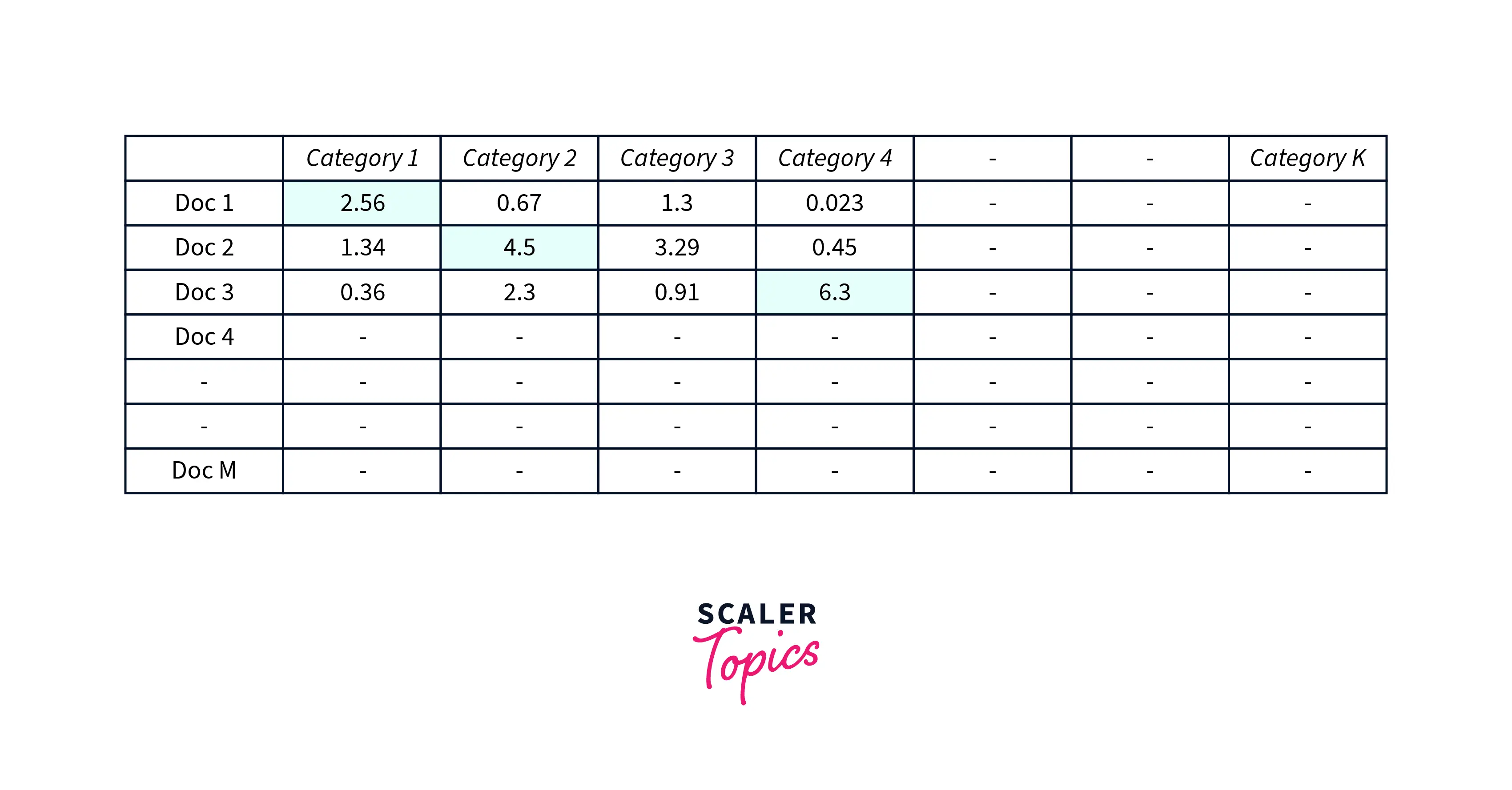
e.g. doc 1 strongly belongs to Category 1 similarly doc 3 strongly belongs to Category 4

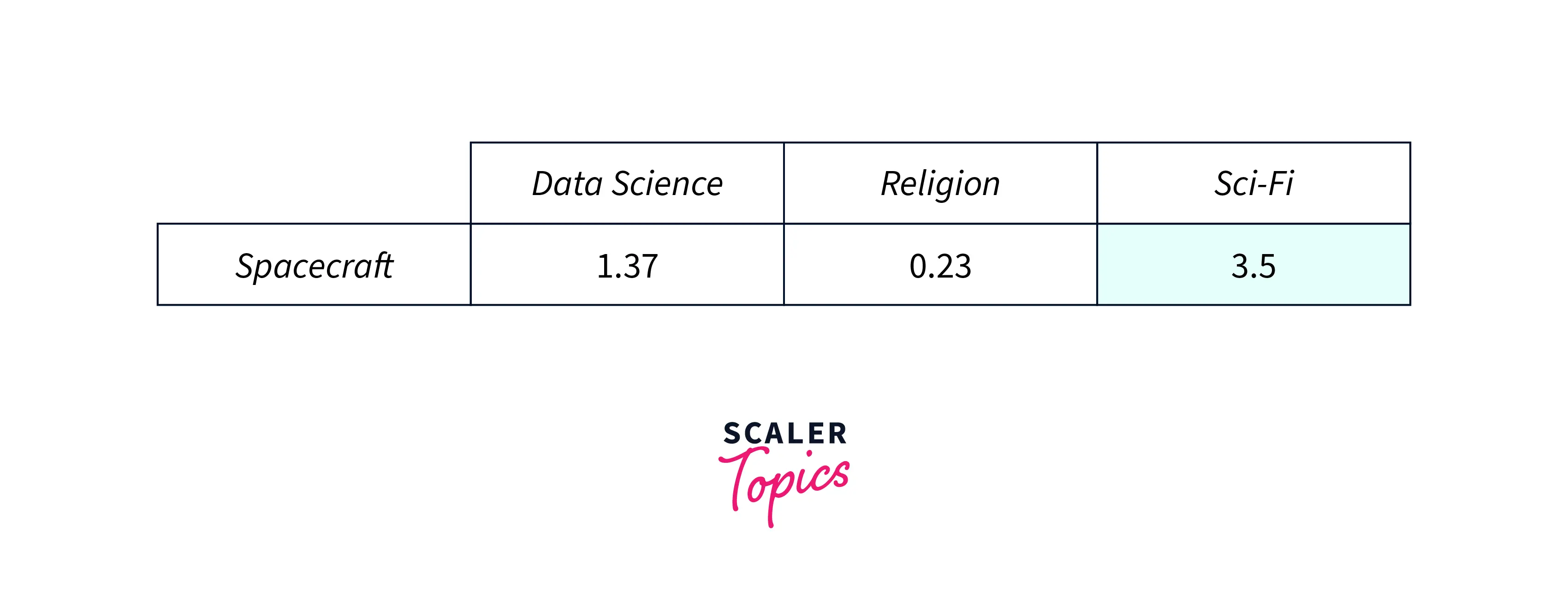
2. A term/word could also strongly belong to a certain category

• This will be represented in a matrix called the term-category matrix (V) and also the term-topic matrix
• Higher cell value indicates that this term is more explained by this category
• For our sample documents this matrix could look like this:

e.g. word/term "spacecraft" is more likely to fall in the "sci-fi" category, therefore its cell value will be higher for the "sci-fi" category

3. How strongly each topic/category represents or explains the data

• This set of information is represented in form of numbers

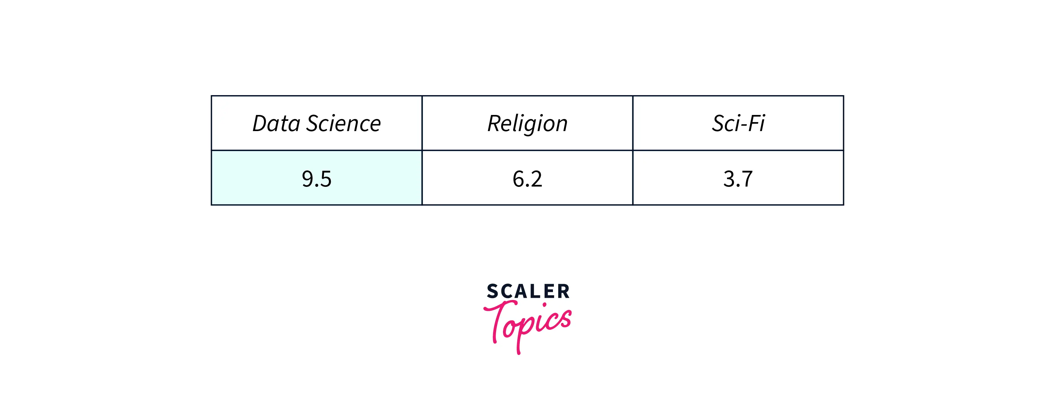
These values tell us what is the relative importance of the hidden topics within our text data. Here we can see that "data science" has a higher weightage and this hidden category explains our text very well.

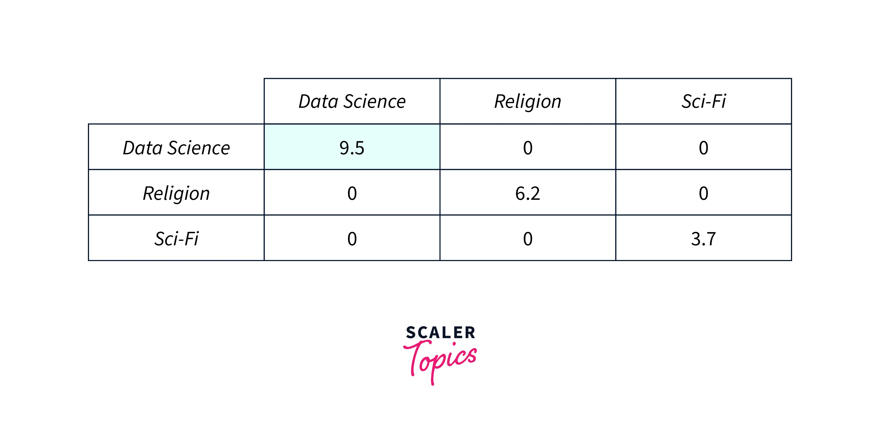
The technical name for this array of numbers is the “singular values”.

In matrix notation (call it Sigma or S matrix) it is represented as a diagonal matrix:

e.g.

If we look closely all three of these matrices (U, V, and S) have one thing in common - hidden topics or hidden categories

The LSA tries to figure out these matrices through SVD.

LSA Matrix Decomposition Intuition

If we call the,

• Document - term matrix as A (size m x n)
• Document - category matrix as U (size m x k)
• Term - category matrix as V (size n x k)
• Singular value matrix as S (k x k)

Then we can see that our original matrix A can be written as a product of U, V, and S.

We have to consider the transposed version of V to follow the matrix multiplication rule, We can write:

A _{m x n} = U _{m x k} * S _{k x k} * V^T _{k x n}

These matrices U, S, and V can be easily found by Singular Value Decomposition (SVD).

If we look closely, the value of k can ideally range from 1 to n. Where "n" is the total number of unique terms across all the documents.

E.g. if we have 20,000 total unique terms we could choose to have 20,000 hidden topics in our data, but that may not be a reasonable approach. We can choose any value of "k" if it seems reasonable.

Let's take a scenario, where we have 100 documents that have 20,000 unique words/terms-

And let's say we choose k = 3 (number of hidden topics that could explain these documents well),

Then the sizes of the above matrices would be :

A _{100 x 20,000} = U _{100 x 3} * S _{3 x 3} * V^T _{3 x 20,000}

So basically we have reduced the dimensions of right-hand side matrices. That's why LSA and SVD are also dimensionality reduction techniques. This is also called a truncated version of SVD.

So technically or mathematically LSA uses a low-rank approximation to the document-term matrix to remove irrelevant information, extract more important relations, and reduce the computational time.

The Math

Reader's Note: You can absolutely SKIP this section if you are not comfortable with Linear Algebra concepts specifically eigenvectors and linear transformations and directly jump onto the coding implementation of LSA.

Now we know that LSA uses SVD for the matrix decomposition. Let's explore a few important aspects of SVD mathematically.

Before we deep dive into a little mathematics of SVD I would highly recommend going through the Essence of Linear Algebra Playlist on Youtube by 3Blue1Brown. This would give you a geometric understanding of matrices, determinants, eigen-stuffs, and more.

Also this Linear Algebra course by Khan Academy would make your linear algebra concepts stronger. The SVD maths is easier to follow if your basics are clear.

SVD Maths

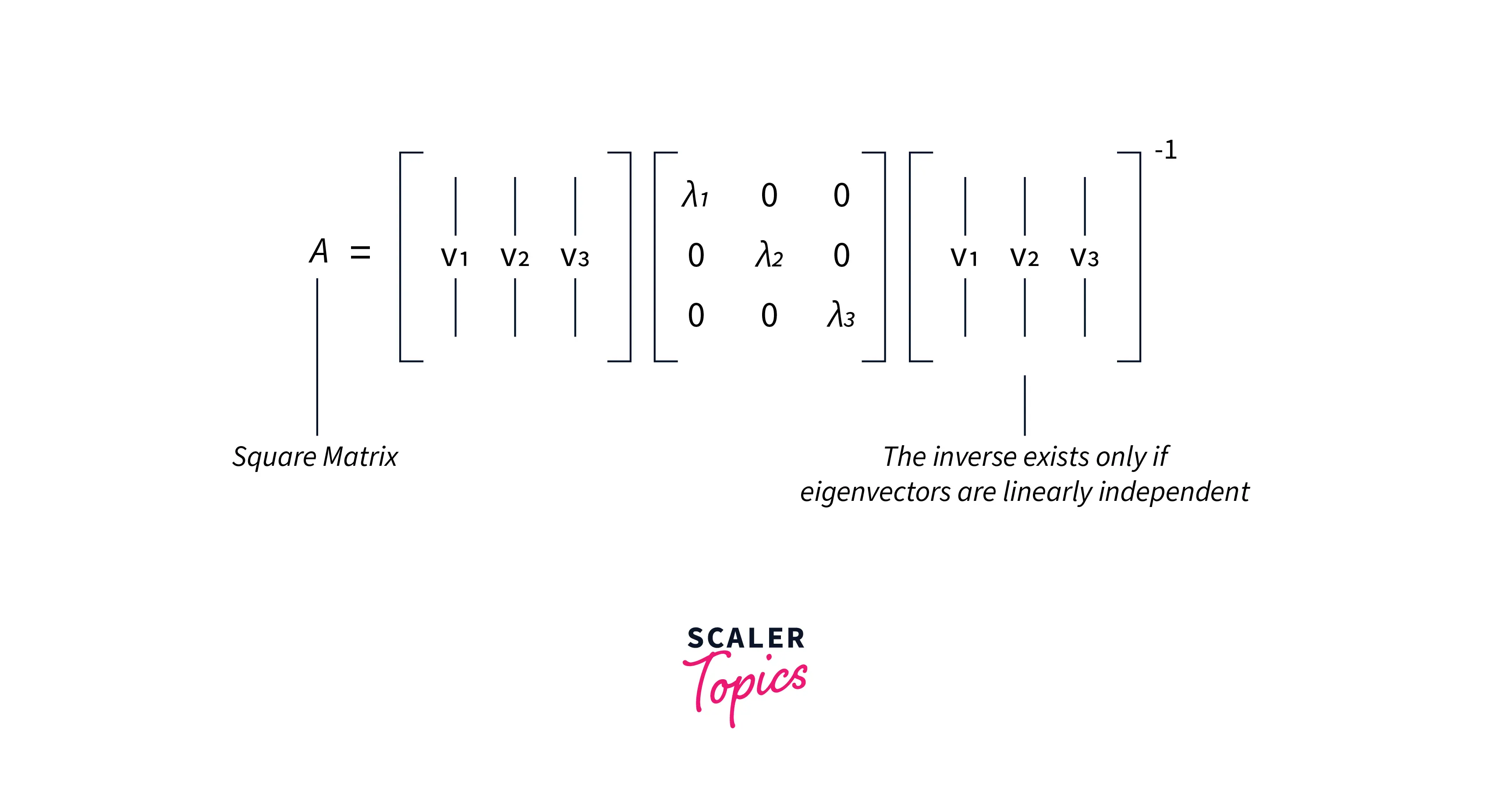
If A is a square n x n matrix it can be decomposed into its eigen vectors and eigen values.

We can write A as :

Where;

• This is possible only if A is a square matrix and A has n linearly independent eigenvectors.

• Consider any m × n matrix A, The matrix AAᵀ and AᵀA will be square metrices of size (m x m) and (n x n) respectively. These matrices have very special properties :

• Both of them are square and symmetrical and their eigenvalues are zero or positive (called positive semidefinite)

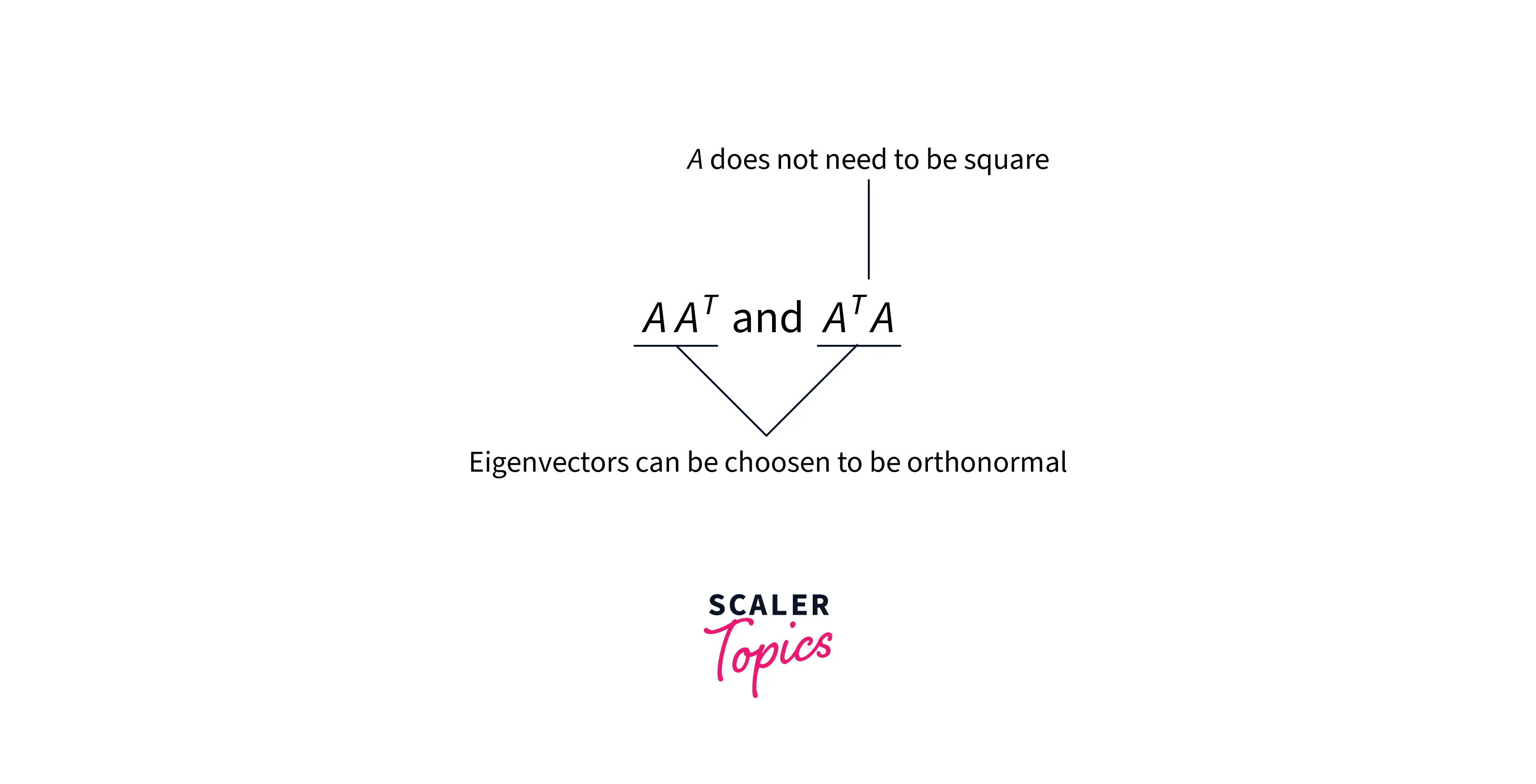
Since they are symmetric, we can leverage properties of symmetric matrices and we can find their eigenvectors to be orthonormal i.e. perpendicular to each other with unit length.

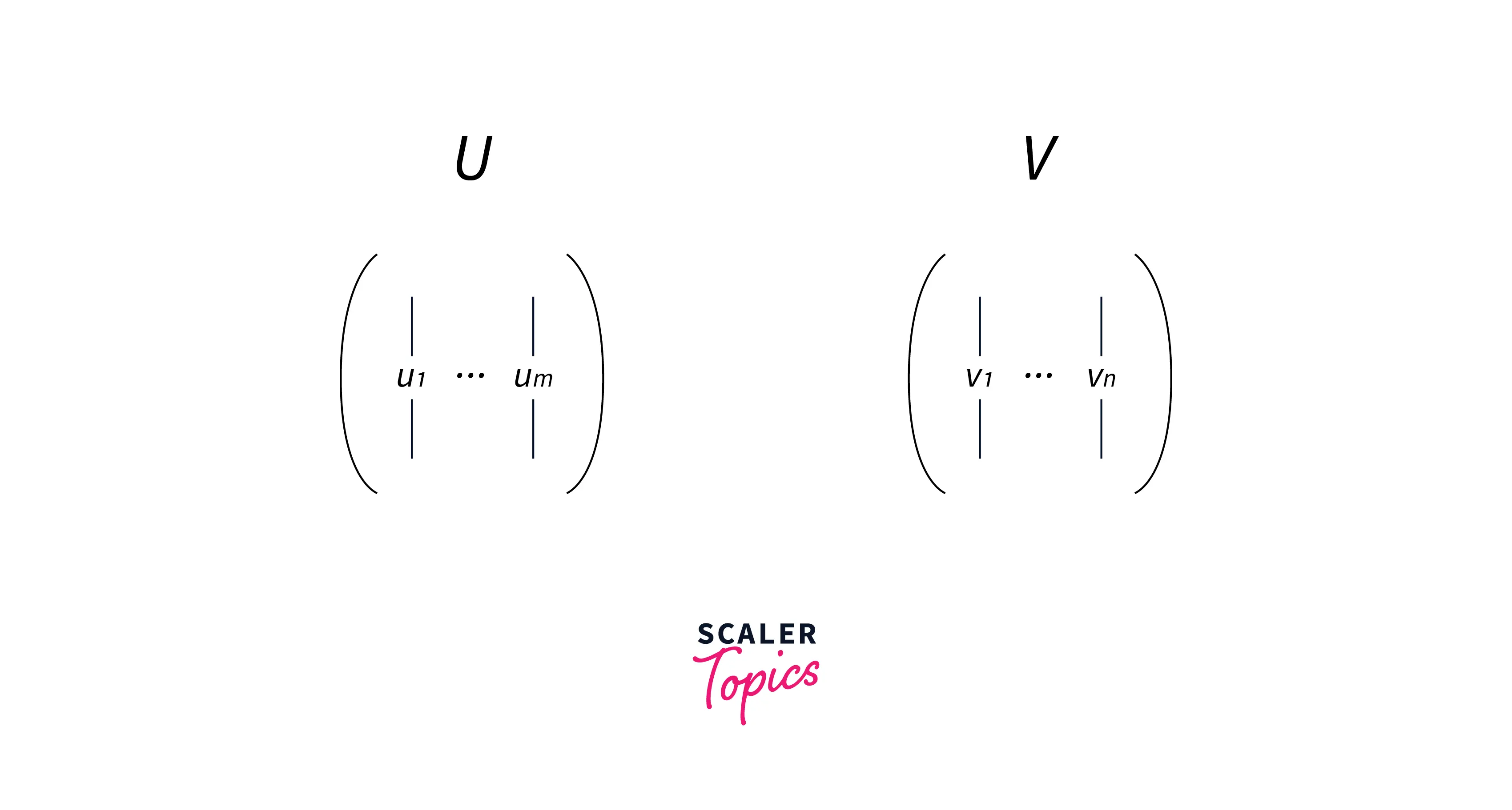
• The Eigenvectors of the matrix AAᵀ and AᵀA are called singular vectors in linear algebra.

Let's represent the set of eigenvectors of AAᵀ as u and the set of eigenvectors of AᵀA as v.

Both of these matrices have the same positive eigenvalues. The square root of these eigenvalues are called singular values.

Representing the set of eigenvectors of these both matrices as U (have m eigenvectors) and V (have n eigenvectors) matrices.

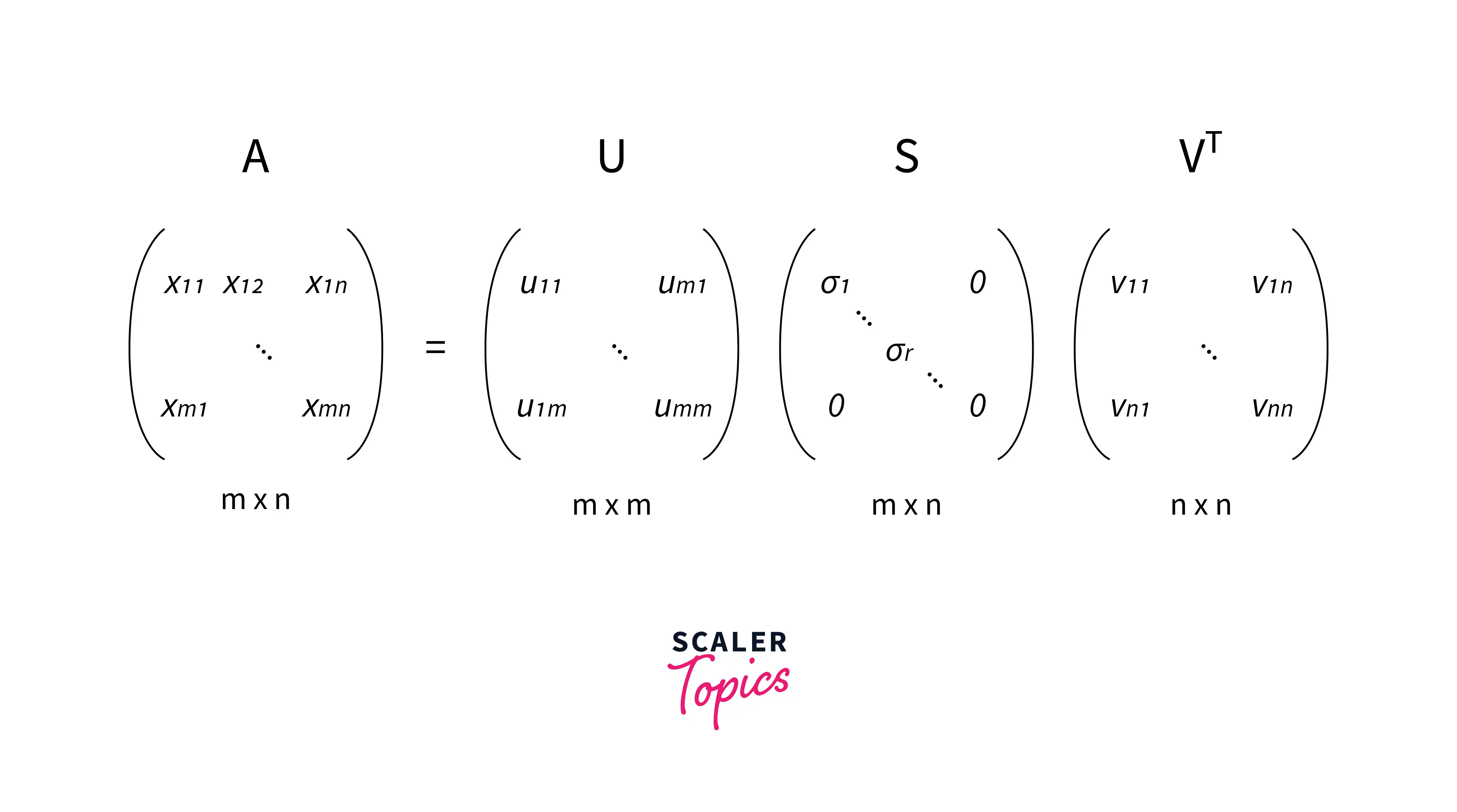
According to the SVD, any matrix A of size (m x n) can be factorized as:

A _{m x n} = U _{m x m} * S _{m x n} * V^T _{n x n}

• Where U and V are orthogonal matrices with orthonormal eigenvectors chosen from AAᵀ and AᵀA respectively.
• S is a diagonal matrix with r elements equal to the square root of the positive eigenvalues of AAᵀ or Aᵀ A (both matrics have the same positive eigenvalues).
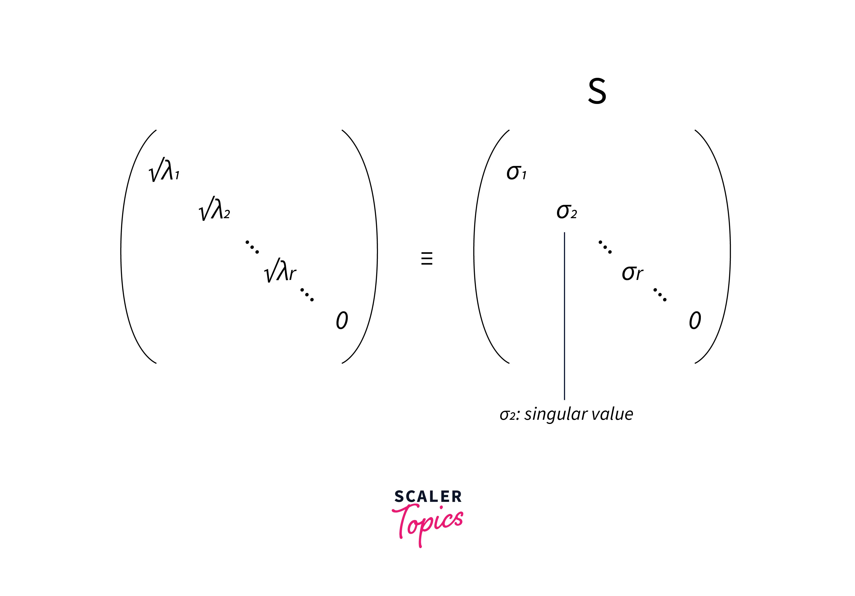
• The diagonal elements of the S matrix are composed of singular values.

where σ_i's are singular values, equal to the square root of eigenvalues λ_i's

σ_i = sqrt(λ_i)

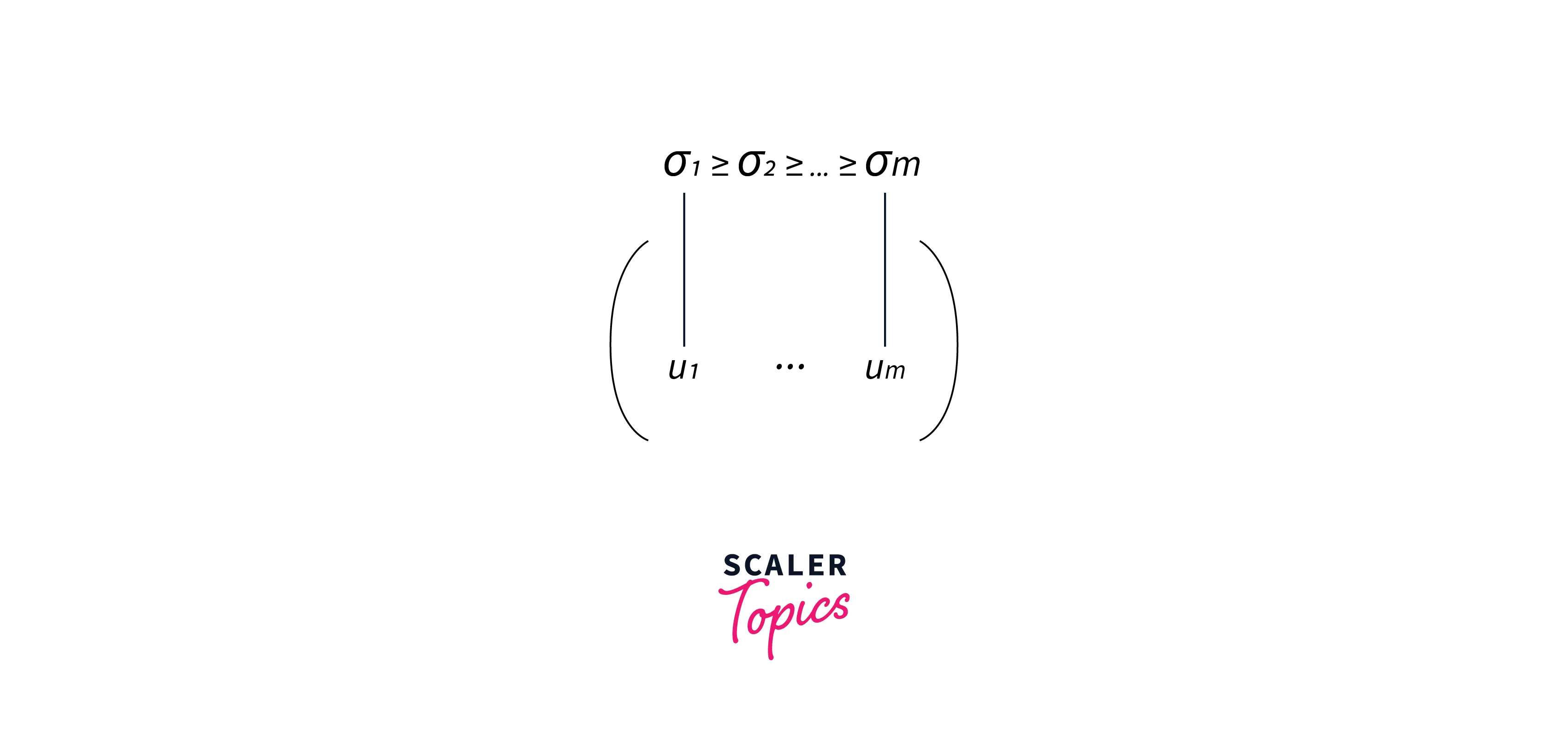
• The eigenvectors inside matrices U and V are ordered according to their corresponding eigenvalues (highest to lowest).

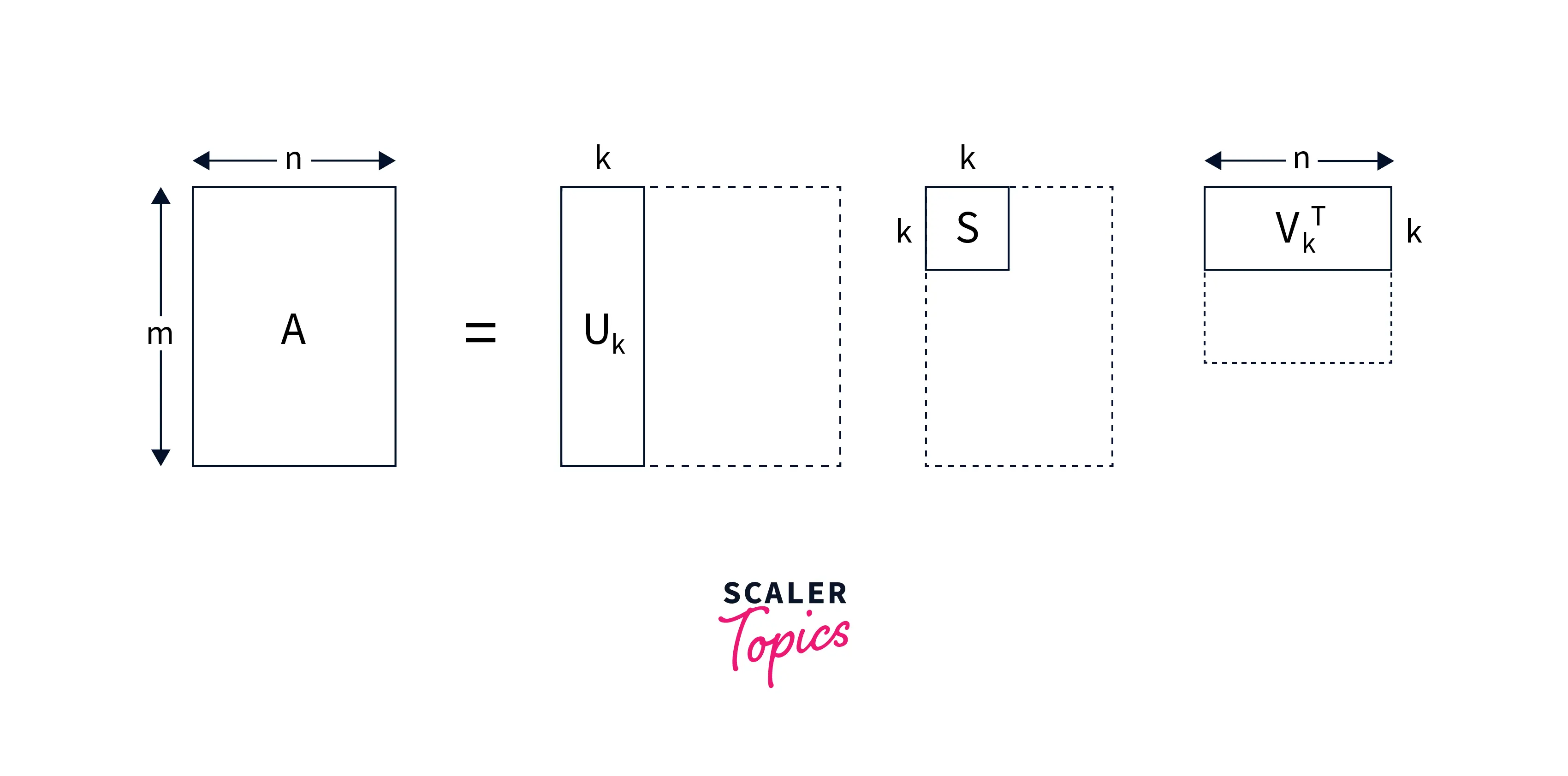
Now we can easily see that If A is our original data matrix we can approximate A as its summation of singular values, eigen vectors multiplication:

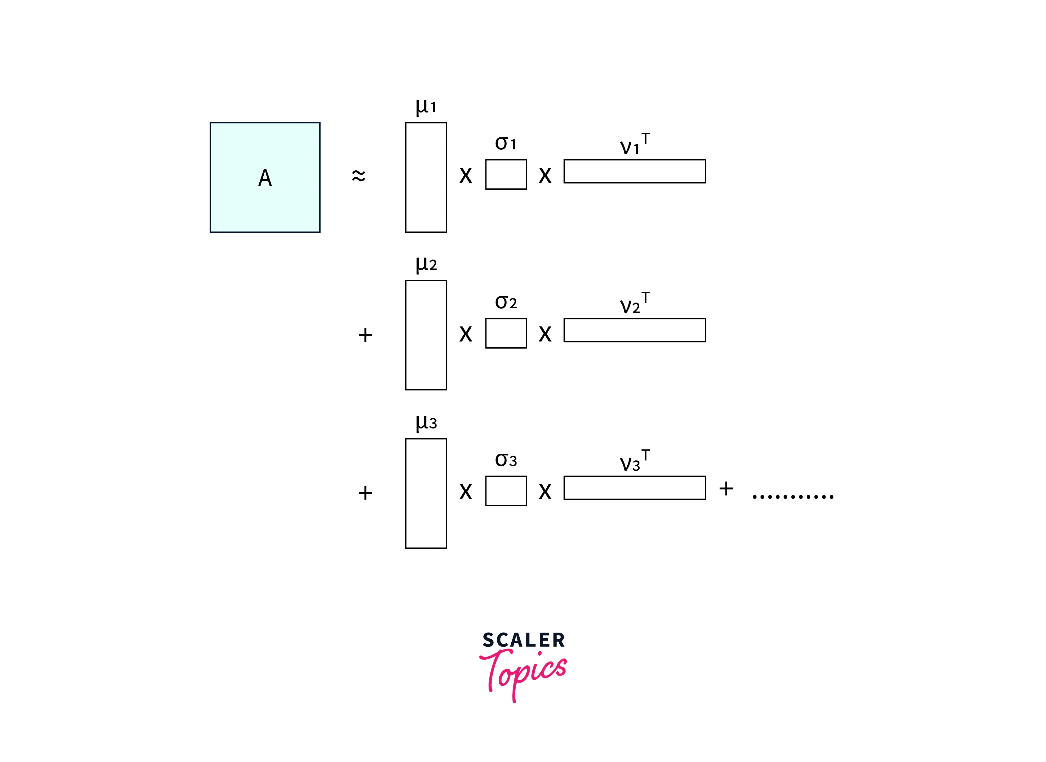
• Previously we had the tall U, the square S and the long 𝑉-transpose matrices.

• Here we are taking the first vertical slice from U (first eigenvector of AAᵀ), weighting (multiplying) all its values by the first singular value, and then, by doing an outer product with the first horizontal slice of 𝑉-transpose (first eigenvector of AᵀA),

• Creating a new matrix with the dimensions of those slices.

• Then we add those products together and we get the original data matrix A.

• If we don’t do the full sum but only complete it partially, we get the truncated version (i.e. till "k" concepts or categories)

LSA Code Implementation

Let's implement LSA using text documents from news articles.

Expected outcome from the algorithm

We will extract important keywords per hidden topics or concepts from the news articles and interpret the output whether these keywords make sense in explaining the hidden concept.

Dataset Explanation

• We will use the raw data collected from news articles.

• This data set is a collection of approximately 20,000 newsgroup documents, partitioned almost evenly across 20 different newsgroups.

• This 20 newsgroups collection has become a popular data set for experiments in text applications of machine learning techniques, such as text classification and text clustering.

More details about the data can be found here : http://qwone.com/~jason/20Newsgroups/

Python Code

Output Interpretation

Let's explore a few keywords from 2 categories identified by the algorithm

Keywords from Category 1

Topic 1:

thanks

windows

card

drive

mail

file

advance

files

software

program

These keywords look like they belong to the Microsoft Windows category

Topic 2:

game

team

year

games

season

players

good

play

hockey

league

These keywords look like they belong to the sports - hockey category

Applications for LSA

Latent Semantic Analysis (LSA) is a Topic Modeling technique that uncovers latent topics and has become a very useful tool while we work on any NLP Problem statement.

Major Applications of LSA include:

• The LSA can be used for dimensionality reduction. We can reduce the vector size drastically from millions to thousands without losing any context or information. As a result, it reduces the computation power and the time taken to perform the computation.

• LSA can also be used for document clustering. As we can see that the LSA assigns topics to each document based on the assigned topic so we can cluster the documents.

• LSA is used in search engine optimization, and Latent Semantic Indexing (LSI) is a term often used in place of Latent Semantic Analysis.

• LSA is also used in Information Retrieval, Given a query of terms, translates it into the low-dimensional space, and finds matching documents.