Non Linear Classification Text in NLP

Pre-requisites

Before learning about the nonlinear classification text in NLP, let us first learn some basics about NLP itself.

• NLP stands for Natural Language Processing. In NLP, we analyze and synthesize the input, and the trained NLP model then predicts the necessary output.
• NLP is the backbone of technologies like Artificial Intelligence and Deep Learning.
• In basic terms, we can say that NLP is nothing but the computer program's ability to process and understand the provided human language.
• The NLP process first converts our input text into a series of tokens (called the Doc object) and then performs several operations on the Doc object.
• A typical NLP process consists of various stages like tokenizer, tagger, lemmatizer, parser, and entity recognizer. In every stage, the input is the Doc object, and the output is the processed Doc.
• Every stage makes some kind of respective change to the Doc object and feeds it to the subsequent stage of the process.

Introduction

Text classification in NLP is a process in which we categorize the text into one or more classes so that the text can be organized, structured, and filtered into any parameter. Some of the reasons for using the text classifications are:

1. Scalability:
   Scalability is the property of a system to handle a growing amount of work by adding resources to the system. Hence, we can scale up and scale down the system according to the input and use case.
2. Consistency:
   A desirable property of a good language understanding model is consistency. It is the ability to make consistent decisions in semantically equivalent contexts, reflecting a systematic ability to generalize in the face of language variability.
3. Speed:
   Speed refers to the reaction time of particular input. A good NLP model which is well-trained can answer queries quite fast.

Some of the most commonly used text classification algorithms are as follows:

1. Linear Support Vector Machine
2. Logistic Regression
3. Naive Bayes

There are mainly two types of classification in the world of neural networks, machine learning and NLP i.e. linear classification and non-linear classification.

In linear text classification, we categorize the set of data into a discrete class depending on the linear combination of its explanatory variables. An example of linear text classification can be Support Vector Machine.

On the other hand, in non-Linear text classification, we categorize the non-linearly separable instances. An example of non-linear text classification can be neural networks.

Let us now dive deep into the non-linear classification in detail in the next sections.

What is Non-Linear Classification?

The classification of the instances that are non-linearly separable is known as non-linear classification. Suppose that we have two classes (X and O) in a data set. Now, if we want to separate these two classes, then we cannot separate them by just drawing an arbitrary straight line (like we used to do in a linear classification). So, to separate these two classes, we perform the precision-wise classification boundaries (linear or non-linear).

Feed-forward Architecture

Before getting deep into the feed-forward architecture, let us briefly discuss neural networks. Neural networks, also known as artificial neural networks (ANNs) or simulated neural networks (SNNs), are a subset of machine learning and are at the heart of deep learning algorithms. Their name and structure are inspired by the human brain, mimicking the way that biological neurons signal to one another. Artificial neural networks (ANNs) are comprised of node layers containing an input layer, one or more hidden layers, and an output layer. Each node, or artificial neuron, connects to another and has an associated weight and threshold. If the output of any individual node is above the specified threshold value, that node is activated, sending data to the next layer of the network. Otherwise, no data is passed along to the next layer of the network.

Architecture is comprised of various connected nodes. These nodes are arranged in a certain format to generate a particular architecture. A feed-forward architecture only processes the input data in one direction. The data travels in only one direction, and the data flow does not return (no backward flow).

In the case of a feed-forward neural network, each neuron present in the network acts similarly to the linear regression. At the end of the neuron, an activation function is used. Each neuron of the feed-forward neural network works on its weighted vector. An example of a feedforward Neural Network is given below. It is a directed acyclic Graph which means that there are no feedback connections or loops in the network. It has an input layer, an output layer, and a hidden layer. In general, there can be multiple hidden layers.

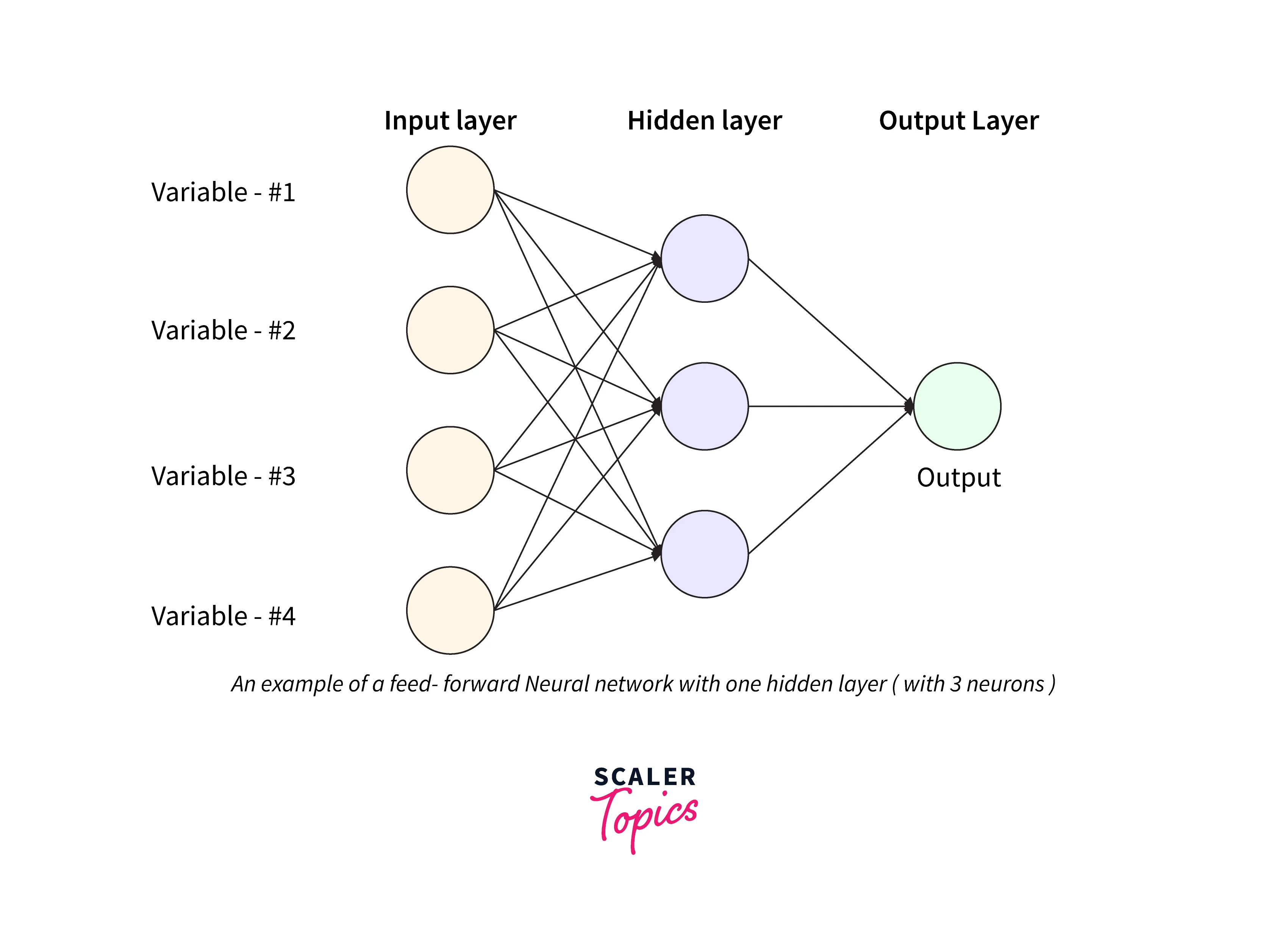
A feed-forward neural network has some of the routes in the cycled form, and its entire nodes are connected circularly, yet it is one of the simplest types of a neural network as the input only flows in a single direction. Also, it is one of the most primarily developed neural networks. A feed-forward neural network contains an input layer, an output layer, and a hidden layer.

Activation Functions

As the name suggests, an activation function checks whether a neuron of the neural network is still active or not. In a more theoretical term, we can say that this function decides or checks whether the input to a particular neuron is important or not. The main aim of using an activation function is to decide the activeness of a neuron as well as to derive the output or result out of the provided set of inputs.

As we have discussed earlier that a neural network is a collection of numerous neurons arranged in the order of the input layer, then the hidden layer, and finally, the output layer. A layer is fed with inputs and weight, and we generally denote the input with the symbol x, and weights with the symbol w. So, an activation function transforms the weighted input from the input layer node to the hidden layer node and finally to the output layer node. Please refer to the diagram provided below for more clarity.

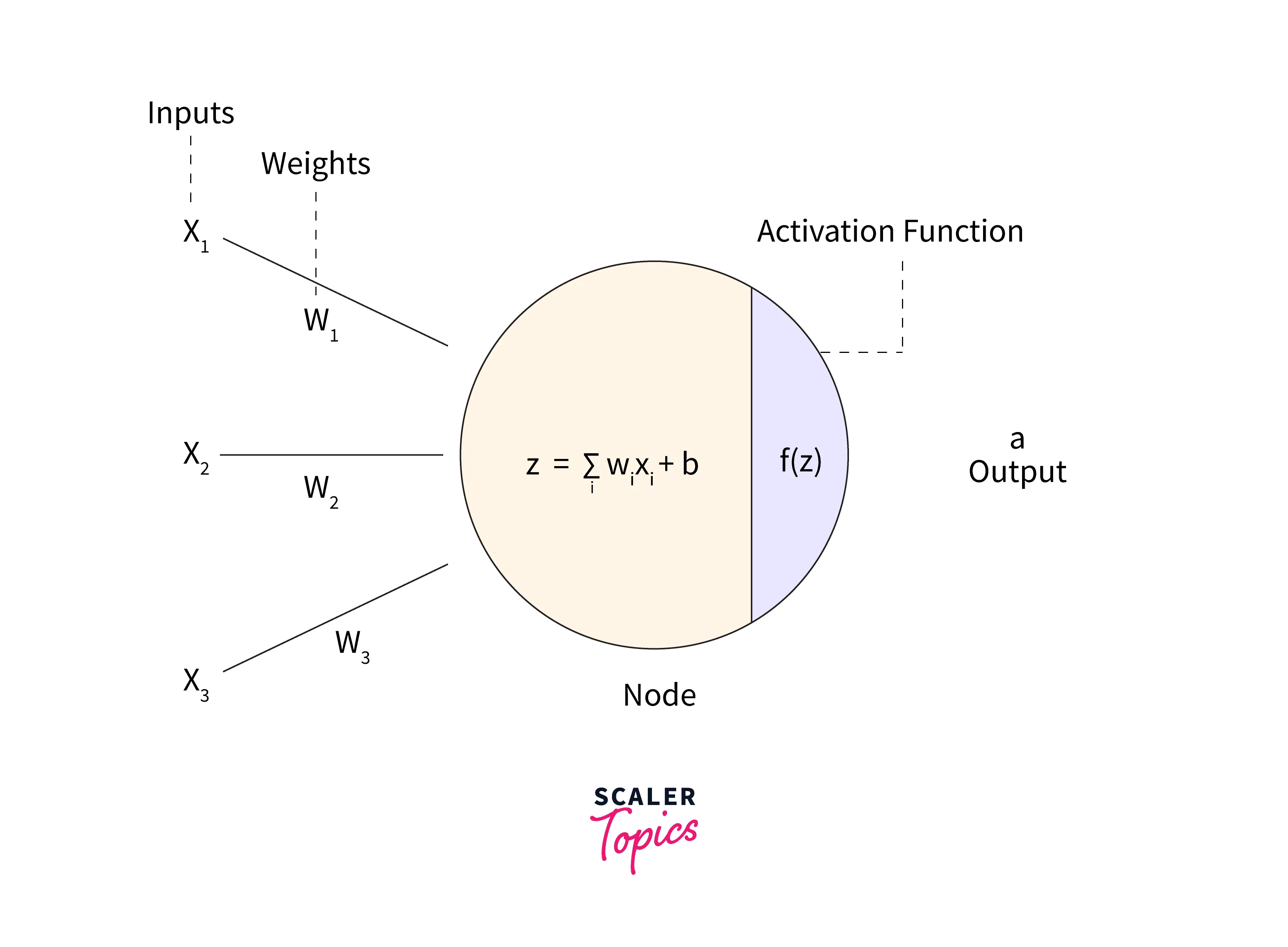
So far, we have discussed a lot about the activation function. But why do we need an activation function? Well, an activation function helps in the greater performance of a neural network by adding some non-linearity to the neural networks. It adds non-linearity by adding a step in the node computation, but this computation is worth doing.

There are mainly seven types of activation functions.

1. Binary Step Function.
2. Linear Activation Function.
3. Non-Linear Activation Function.
4. Sigmoid or Logistic Activation Function.
5. Rectified Linear Unit Activation Function.
6. Leaky ReLU.
7. Tanh or hyperbolic tangent Activation Function.

Training the Neural Networks

Let us now learn how we can train a neural network. For the training of neural networks, we generally use an algorithm i.e., Gradient Descent or GD. The gradient descent algorithm uses the input data sets and cost function to train the model iteratively over time. Our main aim is to minimize the loss or cost function in each iteration by finding the local maxima or minima of the provided function.

The neural network learns from the gradient descent function in batches. The overall formula for the training is:

where

• $\eta^{(t)}$ is the learning rate at update $t$
• $\ell^{(i)}$ is the loss on instance (minibatch) $i$
• $\nabla_{\theta_k^{(z \rightarrow y)}} \ell^{(i)}$ is the gradient of the loss concerning the output weights $\theta_k^{(z \rightarrow y)}$

There is another algorithm that comes into the picture when we are training the neural network model i.e., Back-propagation. As we have previously discussed that a gradient descent function trains the model. Now, when some error is generated in the training of the model, the error is again fed to the input layer in a reverse manner so now when the model can get to know the error. Thus it improves the next iteration. So, in a more theoretical way, we can define Back-propagation as an algorithm that propagates the error from the output node to the input node in a backward manner. In simpler terms, this algorithm is just backward propagation of the error generated in the output layer. Backpropagation is also known as backward propagation.

The algorithm uses the input node, hidden layer node, output layer nodes, and other important parameters to construct a directed acyclic graph. Please refer to the diagram provided below for more clarity.

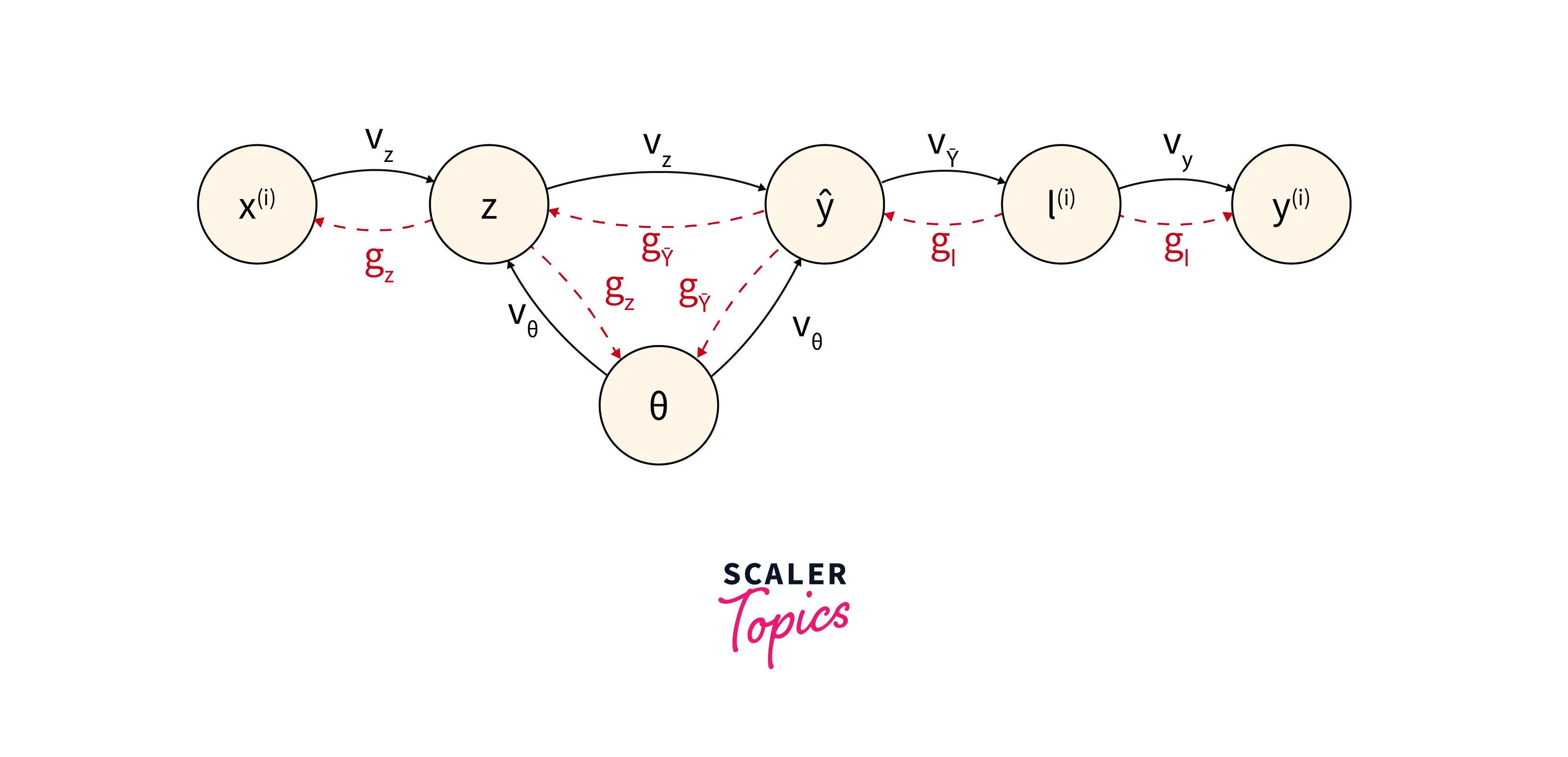
In the above diagram, the value Vx goes from the parents to the children nodes (in a forward pass). On the other hand, the gradient gz goes from the children's node to the parent node (in a backward pass). As we can see that gradients are taking place one after the other, thus it implements a chain rule.

Representing Text for Non-linear Classification

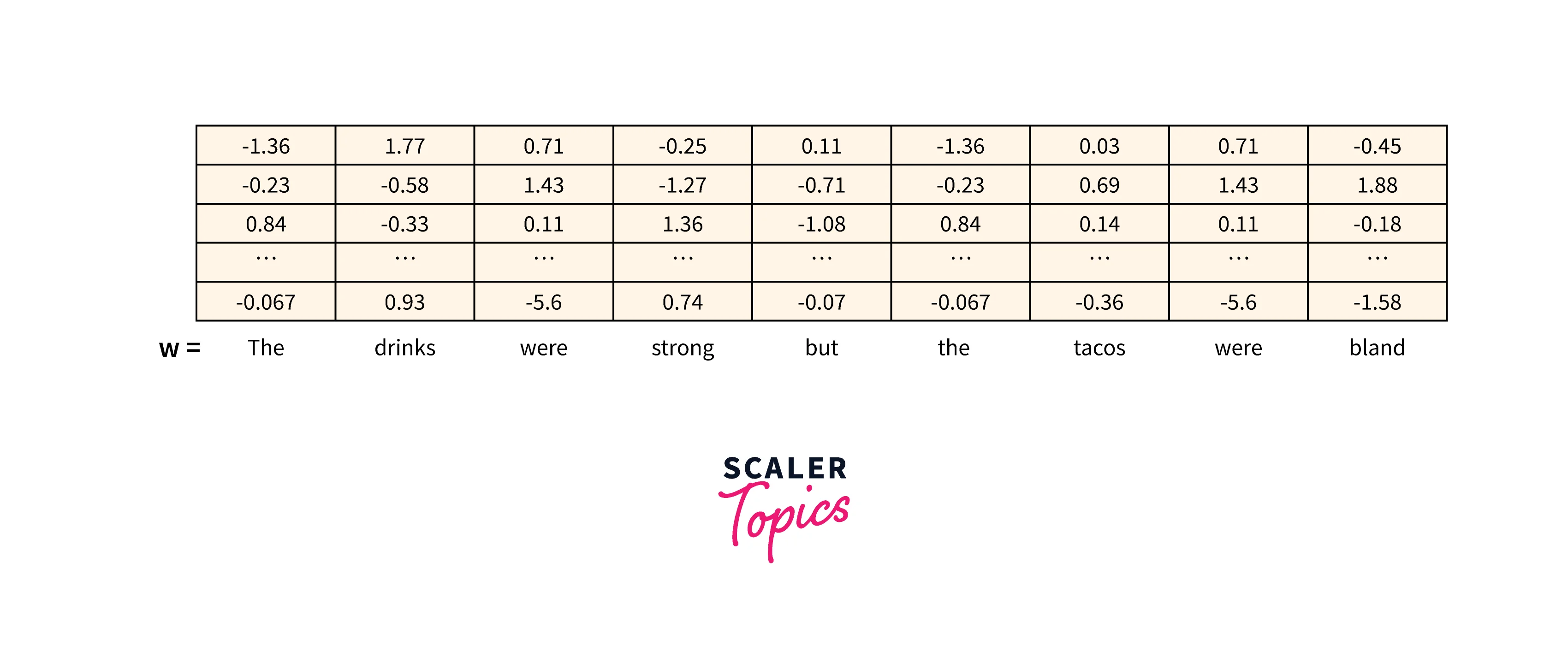
In the learning of neural networks, a text is a sequence of various tokens. A token is usually represented with the letter w. So we can represent a text as:

These tokens are then converted into a bag of words for further transformation, but during the conversion of tokens to the bag of words, the context of the text is somewhat lost. So, we use a look-up layer that can compute the embeddings or real-valued vectors for each of the associated types. For example, we can create a look-up layer like:

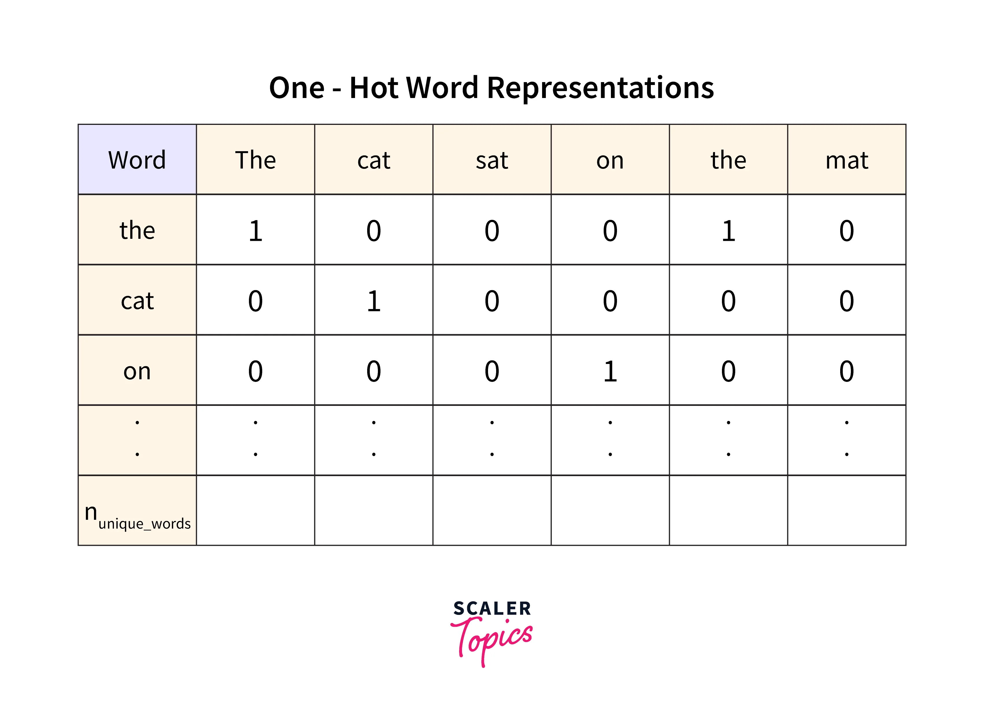
This operation gives rise to a value matrix. Please refer to the image provided below to see a sample matrix.

Evaluation of Non-linear Classifiers

To predict the future performance of the neural network and the created model, we perform the evaluation. Since we have trained our model on some data sets, but the model will have to work on unseen data, an evaluation is necessary. Let us see how we evaluate a model or a neural network.

Beyond "right" and "wrong"

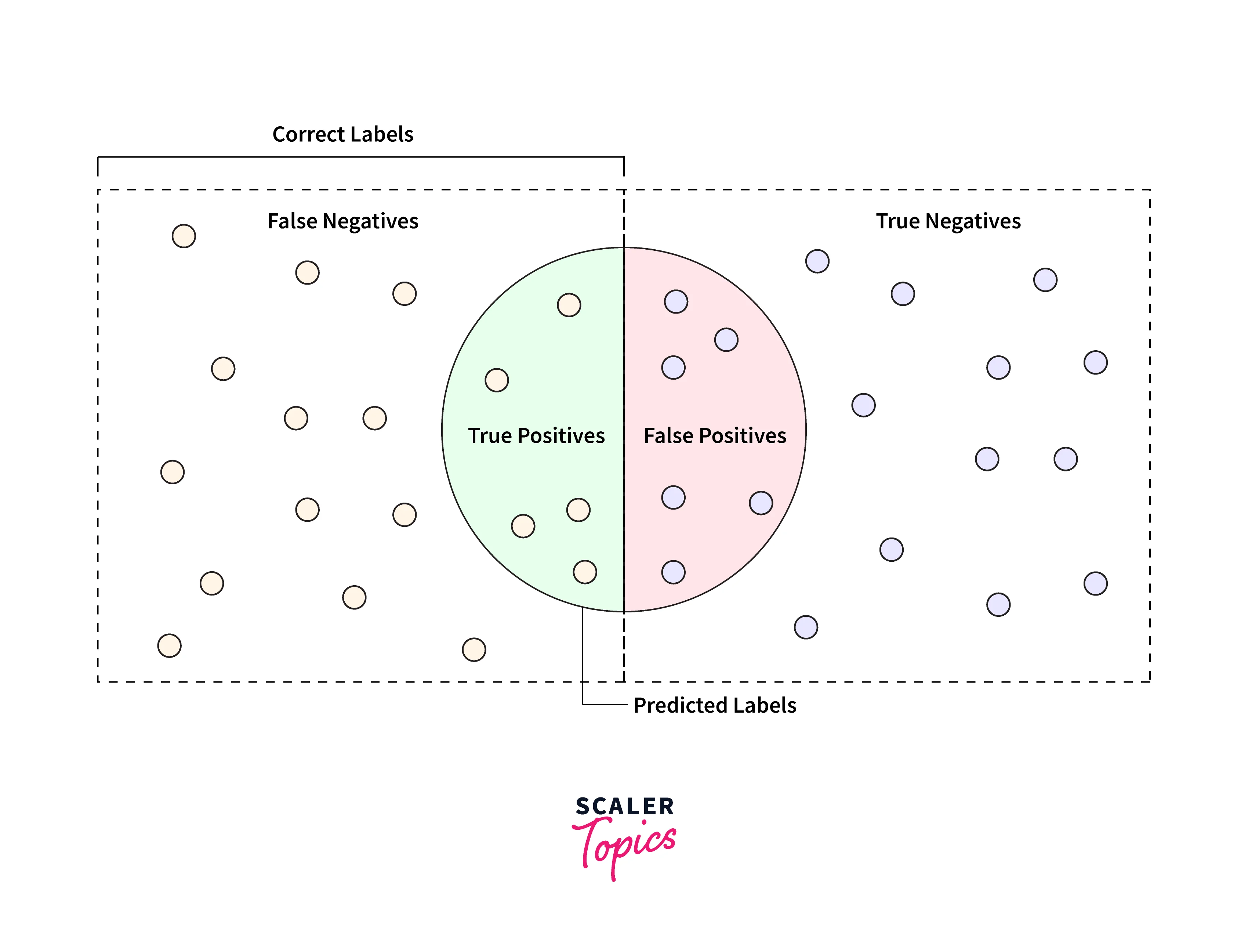
Wrong and right are used in the evaluation of a non-linear classifier. For any provided label, we can have two ways of wrong:

1. False Positive:
   It happens when the system is incorrectly predicting the label.
2. False Negative:
   It happens when the system is incorrectly failing to predict the label.

Similar to the wrong, we have two ways of right:

1. True Positive:
   It happens when the system is correctly predicting the label.
2. True Negative:
   It happens when the system is predicting the label, which is not of any instance type.

Please refer to the diagram provided below for more clarity.

Accuracy

Accuracy is a very simple evaluation technique that checks how often our classifier is right. The formula for calculating the classifier is:

Precision & Recall

Precision and recall are also quite important evaluation techniques (computed mathematically) of neural networks' correctness.

The recall is defined as the fraction of the positive instances to the instances that are correctly classified. On the other hand, we can define precision as the fraction of the positive predictions to the total number of classified positive samples (whether incorrect or correct).

Let us now look at both formulas.

For example, in the below-mentioned scenario, the model correctly classified two positive samples while incorrectly classifying one negative sample as positive.

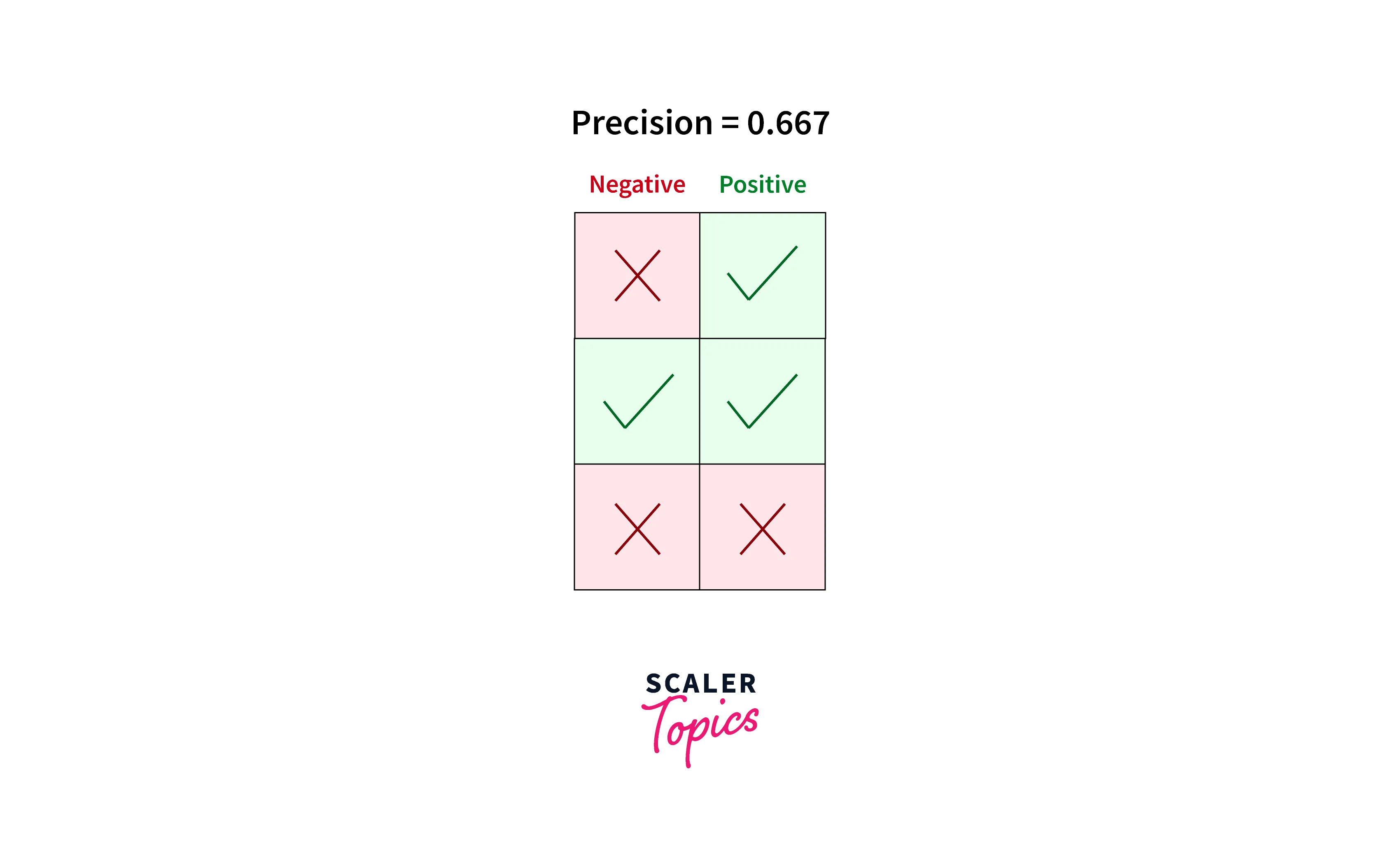
Hence, according to the precision formula, Precision = TP/TP+FP

Example of recall:

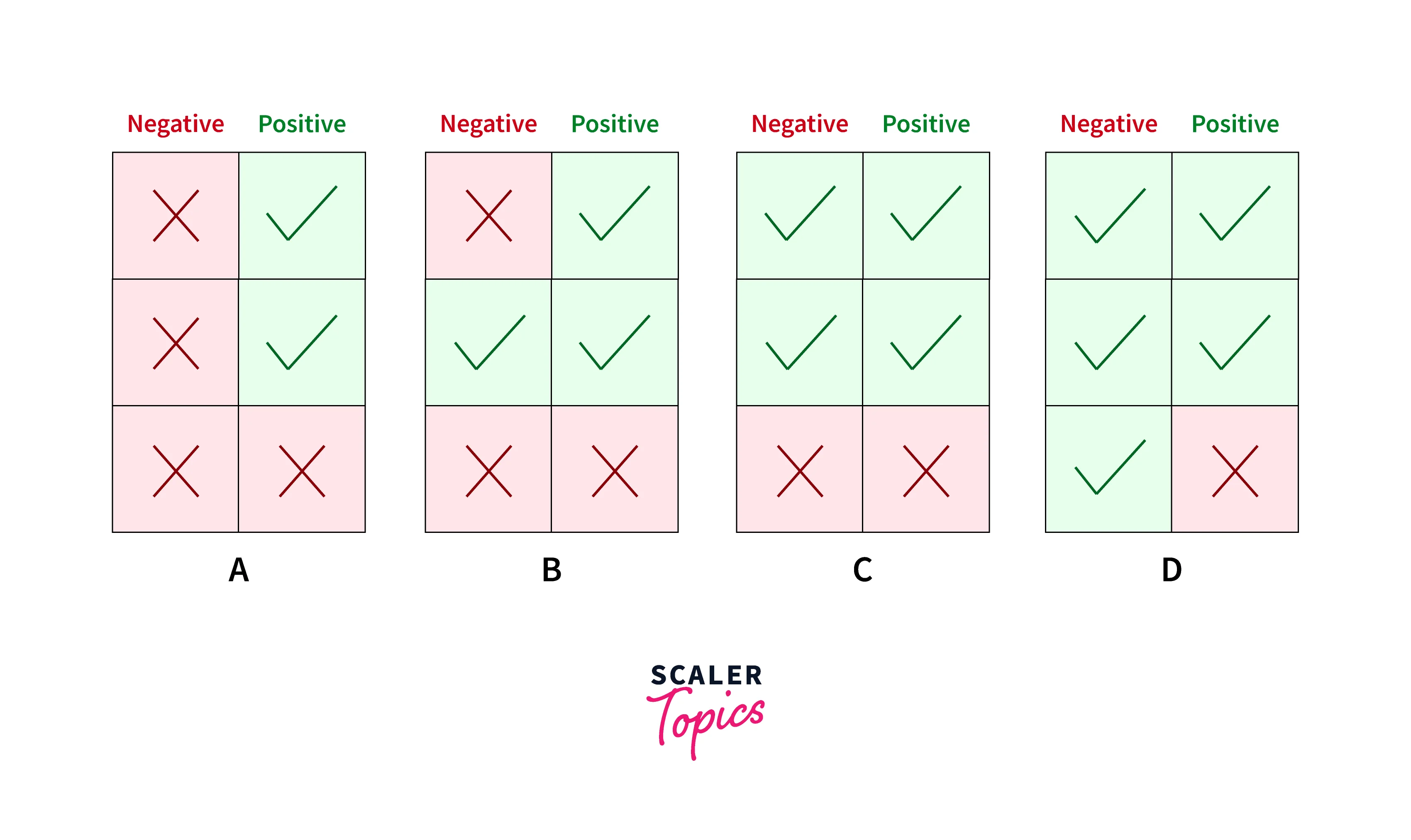
In the above example, we are calculating the recall with four different cases where each case has the same Recall as 0.667 but differs in the classification of negative samples.

Combining Precision and Recall

When we combine the results of precision and recall, then a very important measure is generated i.e. F1 score. The F1 measure is used to calculate the average of precision and recall. The F1 score is simply the harmonic mean of precision and recall.

The F1 score measures the rate performance of our neural network using the statistical formula.

The overall formula for calculating the F1 score is:

Please keep a note that the more value of F1 means a more accurate model.

The F1 scores can range from $0$ to $1$, with $1$ representing a model that perfectly classifies each observation into the correct class and $0$ representing a model that is unable to classify any observation into the correct class.