PLSA – Probabilistic Latent Semantic Analysis

Introduction to PLSA

Probabilistic latent semantic analysis, as the name indicates, was inspired by latent semantic analysis. Both can be used for topic modeling in NLP. Topic modeling refers to the task of identifying topics that best describes a set of documents.

The main goal of PLSA is to find a probabilistic model with latent or hidden topics that can generate the data we observe in our document-term matrix. In mathematical terms, we want a model P(D, W) such that for any document d and word w in the corpus, P(d,w) corresponds to that entry in the document-term matrix.

We want something very similar to LSA but that uses probabilities. Hence, statisticians developed a straightforward model once they knew the idea and the objective.

PLSA Model: Intuition and Maths

The PLSA model can be understood in two different ways. Let's look at the two models and discuss them with an intuitive approach - latent variable model and matrix factorization.

Latent Variable Model

We had the idea that our topics are distributions of words and our documents have a probability distribution over the topics; if we multiply these probabilities, we get a conditional type of probability that will give us a word distribution of documents P(w,d).

So this is what we want to have.

Here,

Our document contains words, and we assume this is a kind of random observation, so the probability of observing a word in a particular document should be the product of the probability of this particular document P(d) and sum over all the topics $\sum_{t}$ and in each topic we have the conditional distribution of the words given the topic P(w|t) and the topic given our documents distribution P(t|d).

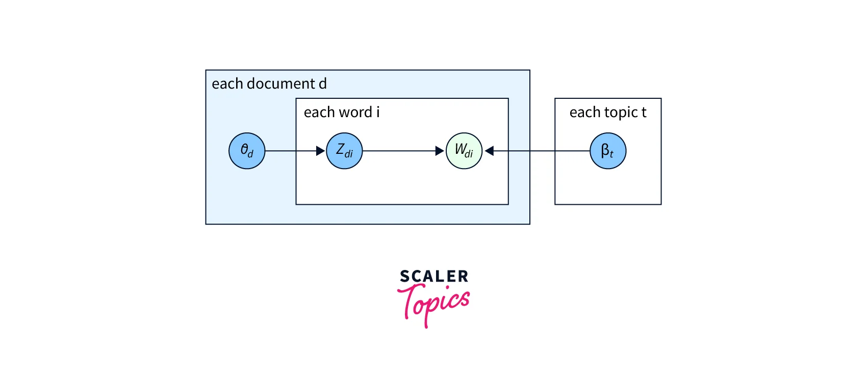
Let's understand this above equation graphically for much better intuition:

• Each document has the topic distribution: $\theta_{d}$

• Each topic has the word distribution: $\beta_{t}$

• For each word z_di in the document d, it belongs to some topic that we drew from the topic distribution $\theta_{d}$,

  • So a popular topic is drawn, or an important topic is drawn more often, and a smaller topic is drawn less often.

• And for each of these topics, we get a word w_di, and that depends on the word distribution of the topics $\beta_{t}$.

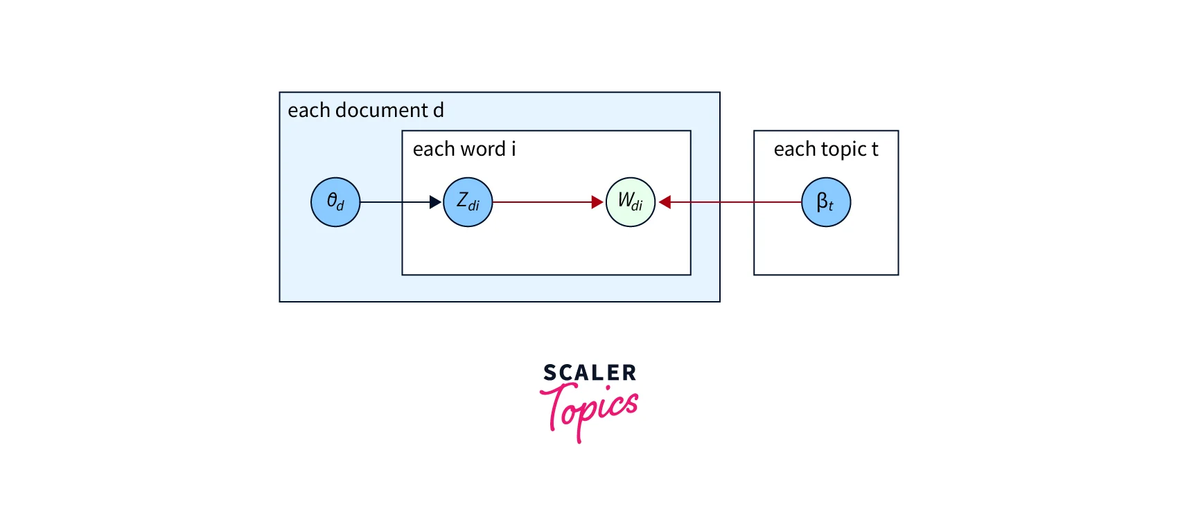
• So once we have these two incoming arrows, we need to consider the combination of these two.

  

• For example, z_di is an indicator variable that says this particular word w_di belongs to topic 5, and for topic 5, we have word distribution coming from $\beta_{5}$, and the word distribution would say that 10% of the words in this topic are from word w_di

• Now we can combine all of this into a probability of the entire corpus, i.e., how likely is the data that we have given our current model, and then we can try to optimize this.

• And optimizing means that we have to optimize our hidden variables because the data that we already have is observed (we cannot change the words of the documents).

• Mathematically it is represented as:

  $P(D) = \Pi_d\Pi_{W_{di}}\Sigma_t\theta_{d,t}\beta_{t,w_{di}}$

  This means how likely is the entire corpus data that we have given our current model and then we can try to optimize the above equation

• And optimizing means that we have to optimize our hidden variables because the data we have is the observed data, and we cannot change the words of the documents, but we can optimize the distribution of topics for each word

Considering PLSA as a generative model:

In literature, PLSA is often called a generative model. But PLSA is not considered to be a fully generative model because the documents (consisting of words) may not make sense due to words disorder (jumbled words)

Let us explain what the generative model means:

We assume:

1. For every topic t, we sample word distribution $\beta_{t}$

2. For every document d, we sample a random topic distribution $\theta_{t}$

3. Given these and given the length of the document l (number of words in a document), For every document d, generate l words, i = 1 to l

   • Sample a topic z_di from the given topic distribution $\theta_{t}$ e.g. picking a random sample of topics from multinomial topic distribution
   • Now we know that the word belongs to a particular topic, e.g., topic 5, So we can take the topic distribution of topic - 5, which is $\beta_{5}$, Sample a word w_di from the above randomly sampled topic distribution $\beta_{5}$

Assumptions of the PLSI model:

1. Word ordering in the document doesn't matter

• As you can see, the document generated this way will be gibberish. They will be completely useless because there need to be ordered to these generated words. Generated words mimic the topics that we have.
• That's why we don't use this to generate documents. But the important takeaway is that PLSA model assumes that the documents are this type of gibberish (random ordering of words) yet strongly indicative of a particular topic.
• The underlying idea is that if we have a document and ask a human to assign the topic he may still be able to do so even if we randomly permute the words in this document. So it will work in many cases; He will still be able to tell that the document probably belongs to the topic politics from these random permutations of words.

2. Conditional Independence

• We assume words and documents are conditionally independent

Likelihood Function of PLSA and Parametrization:

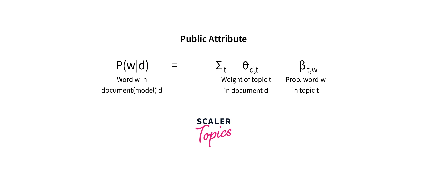
In real data, we have documents, and we observe words in these documents. We need to know what is the likelihood of observing words given a document or if the word w is probable given the document d, i.e., P(w|d)

This likelihood depends on the:

• Topics we have in the document, which we assume are given at this moment

  • denoting this value with $\theta_{d,t}$ which is weight of topic t in the document d.
  • if a topic is very common, this is a high value, and if topic a is very rare, it is a low value.

• And then we take the word distribution of each topic:

  • denoting this value as $\beta_{t,w}$ which is probability of word w in topic t.

• So to compute this probability P(w|d) we multiply $\theta_{d,t}$ and $\beta_{t,w}$ and sum over all t topics.

  

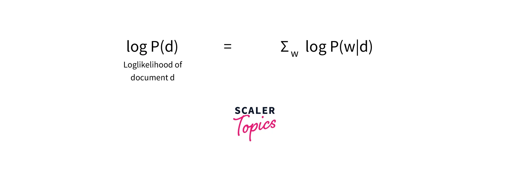
• This probability P(w|d) will be very small, and we may run under the risk of numerical underflow, so we take the log of P(w|d) that would convert the above product expression into a summation.

• Once we have log P(w|d) for each word, we can take summation for all words and can find the log-likelihood of the entire document d as

• Similarly, we can have the log-likelihood for all documents in the corpus D as a summation of the log-likelihoods of all documents d as

  

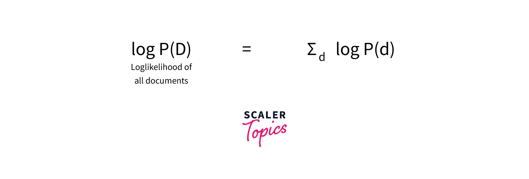
• If we compose the above equation and put values from the previous two equations, we will be having :

  $\log P(D) \quad=\sum_d \sum_w \log \left[\sum_t \theta_{d, t} \beta_{t, w}\right]$

• In this final equation log P(D), we sum over all documents d, sum over all words w in all the documents, and the logarithm of the sum of the $\theta_{d,t}$ weight of topic t in the document d times $\beta_{t,w}$ probability of word w in topic t

This is the function that we want to optimize. We need to maximize this final log-likelihood function.

To achieve this we use Expectation - Maximization (EM) Algorithm.

The discussion of EM algorithms is out of the scope of this article. However, you can explore more about EM algorithms here.

Goal and Outcome of Expectation - Maximization :

Goal:

To optimize parameters $\theta_{d,t}$ and $\beta_{t,w}$.

Outcome:

Once we have optimum values of $\theta_{d,t}$ and $\beta_{t,w}$ we can assign the most probable topic to every word in the document and label the document with the most frequent topic.

Matrix Factorization

The matrix Factorization Model is another alternative way of representing PLSA.

Let's understand this with an example:

Consider a document-term matrix of shape $N × M$, where N represents the number of documents and M represents the dictionary size. The matrix elements represent the counts of the occurrences of a word in a document. The element $((i, j))$ in a matrix represents the frequency of word w_j in the document d_i. We can standardize this matrix with the tf-idf vectorization.

Matrix Factorization breaks this matrix (let's call it A) into lower-dimension matrices with the help of Singular Value Decomposition.

Such that;

A _{m x n} = U _{m x k} _ S _{k x k} _ V^T _{k x n}

where;

• Document - term matrix as A (size m x n)
• Document - topic matrix as U (size m x k)
• Term - topic matrix as V (size n x k)
• Singular value matrix as S (k x k)

Matrix S is a diagonal matrix with diagonal values equal to the square root of the eigenvalues of AAᵀ.

For any given k, we select the first k columns of U, the first k elements of S (Sigma), and the first k rows of V^T. And k represents the number of topics we assume in the document corpus.

Matrix Factorization similarity with PLSA:

This model is not very different from the Probabilistic Latent Variable Model.

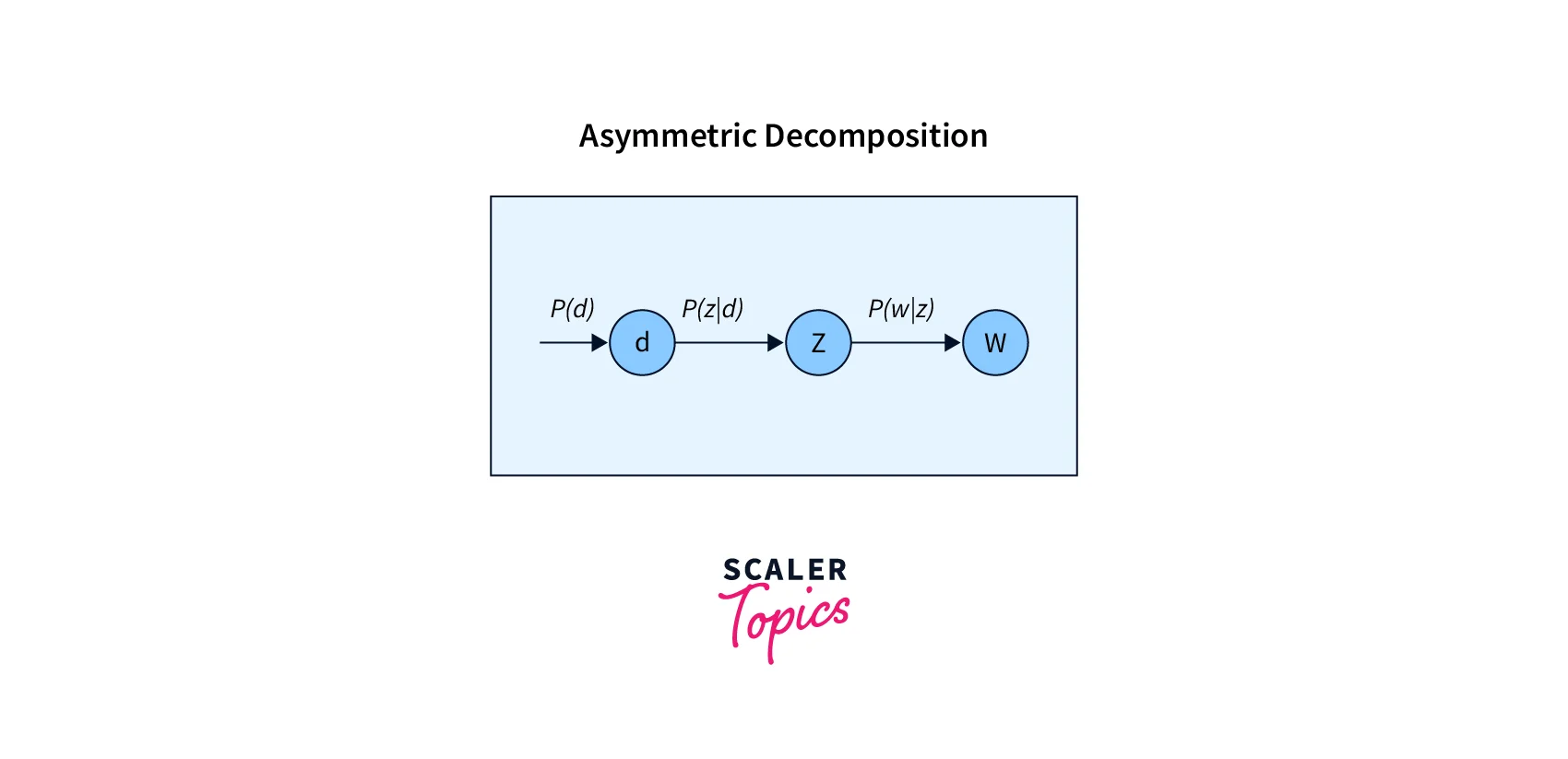
The below equation we have seen in previous sections follows Asymmetric decomposition to generate the word as shown in the image flowchart.

where; z = topic

But, The above equation can be written as:

using Bayes' theorem:

This equation follows Symmetric decomposition to generate documents and words independently, given the topic distribution

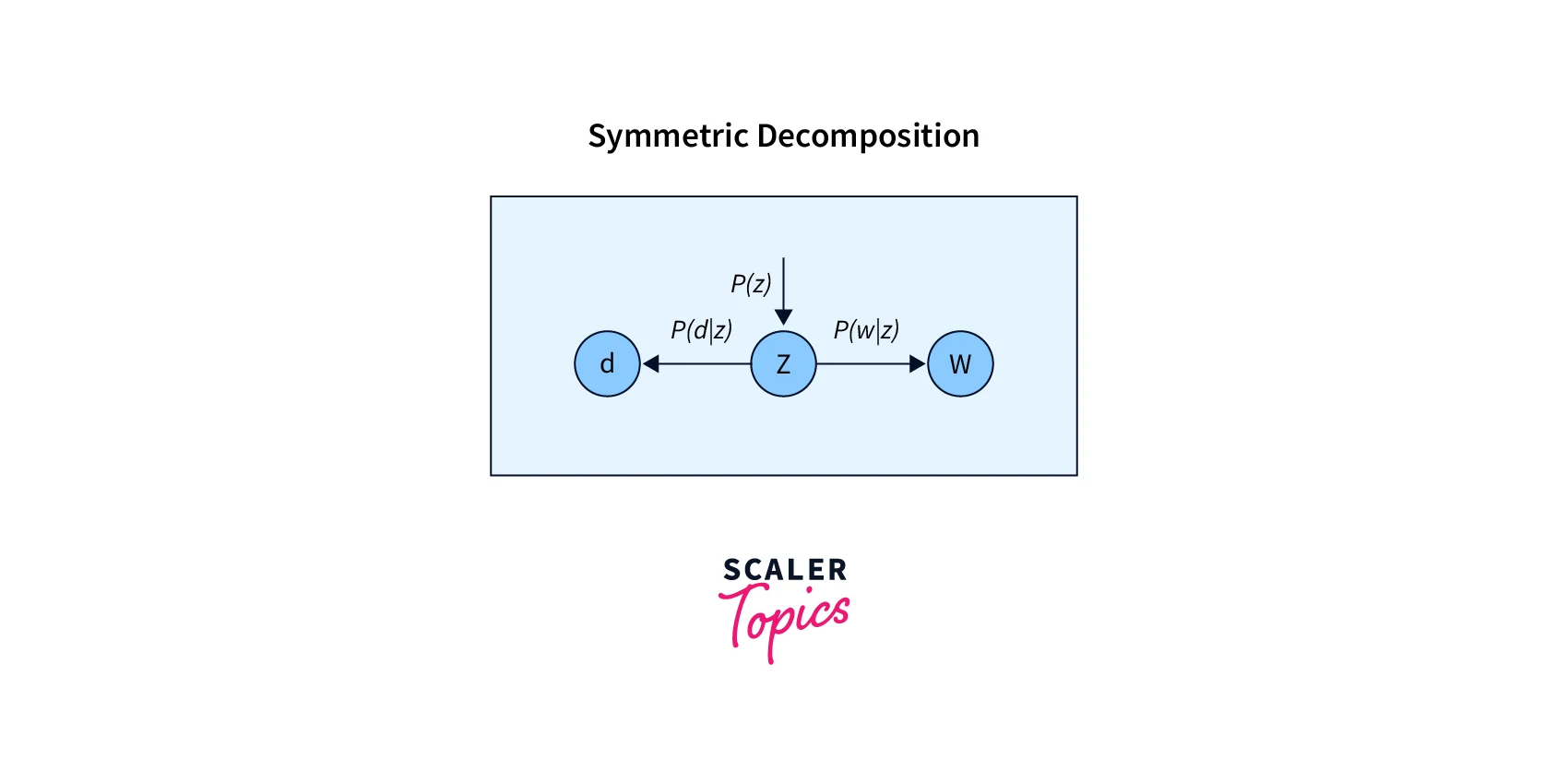
Here,

• P(d|z) : document probabilities given topic
• P(w|z) : word probabilities given topic
• P(z) : topic probabilities

Let's relate these probabilities with the matrices we obtained in the matrix factorization process.

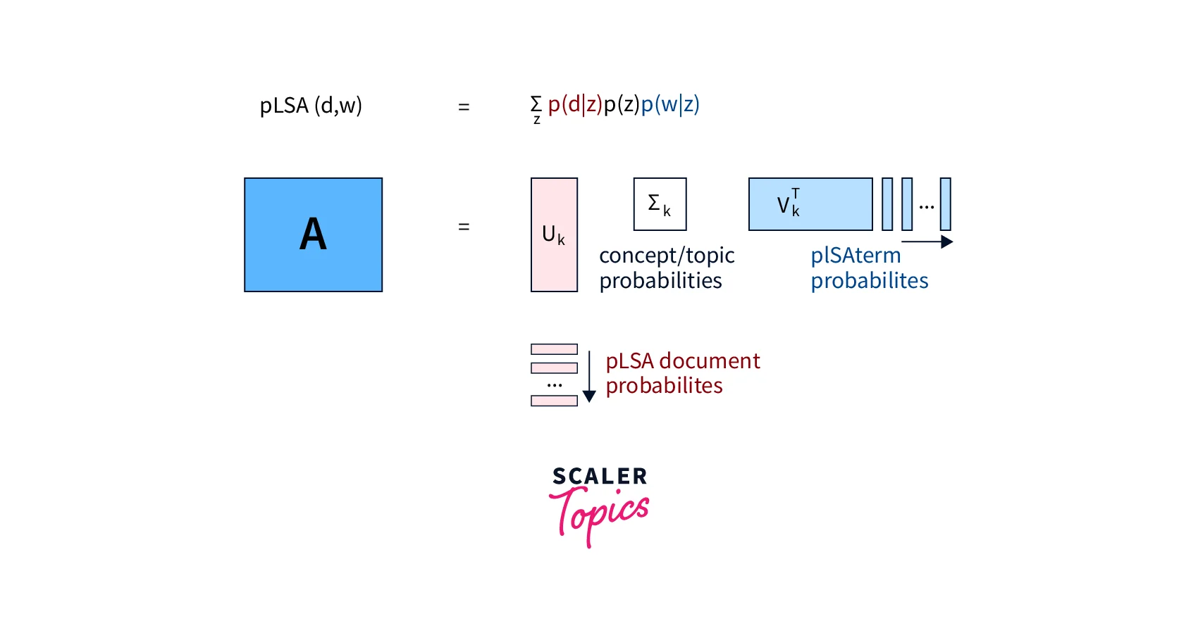
U matrix:
This matrix contains the document probabilities P(d|z)

S matrix:
This is a diagonal matrix that contains the prior probabilities of the topics P(z)

R matrix:
This matrix corresponds to the word probability P(w|z)

Why the Concept of Latent?

Why do we have the concept of "Latent" Semantic Analysis? Here is why the concept of LSA comes up:

• The sparseness problem. The terms that do not occur in a document, get a 0 probability in other approaches making our document term matrices sparse.
• "Unmixing" of superimposed concepts.
• Here, no prior knowledge about concepts is required.

PLSA vs. LSA

While both techniques, PLSA and LSA, can be used for topic modeling, there are a few major differences between them.

• PLSA treats topics as word distributions and uses probabilistic methods, while LSA uses the non-probabilistic method (SVD) for finding hidden topics in the documents

• Since LSA uses SVD, the topic vectors/dimensions are eigenvectors of symmetric matrices. As a result, the topics are assumed to be orthogonal, but in PLSA, topics are allowed to be non-orthogonal (no concept of orthogonality in probability).

Applications for PLSA

• Probabilistic Latent Semantic Analysis (PLSA) is a Topic Modeling technique that uncovers latent topics and has become a very useful tool while we work on any NLP Problem statement
• PLSA can be used for document clustering. As we can see that the PLSA assigns topics to each document based on the assigned topic so we can cluster the documents.
• PLSA is also used in Information Retrieval and many other Machine Learning areas.

Advantages and Disadvantages of PLSA

Advantages:

• PLSA is based on a mixture decomposition derived from a latent class model. This results in a more principled approach with a solid statistics foundation. PLSA approach yields substantial and consistent improvements over SVD-based Latent Semantic Analysis in many cases.

Disadvantages:

• It is reported that probabilistic latent semantic analysis has severe overfitting problems in aspect modeling, so it requires careful implementation.