Text Similarity in NLP
Overview
One of the most important problems in NLP is the similarity of documents. Finding similarities between documents are utilized in a variety of fields, including book and article recommendations, the detection of plagiarism, legal documents, etc.
If two texts define the same notion and are semantically comparable, or if they are identical, we can say that they are similar.
Introduction
Take a look at these pairs of sentences, and observe which pairs are similar and to what extent.
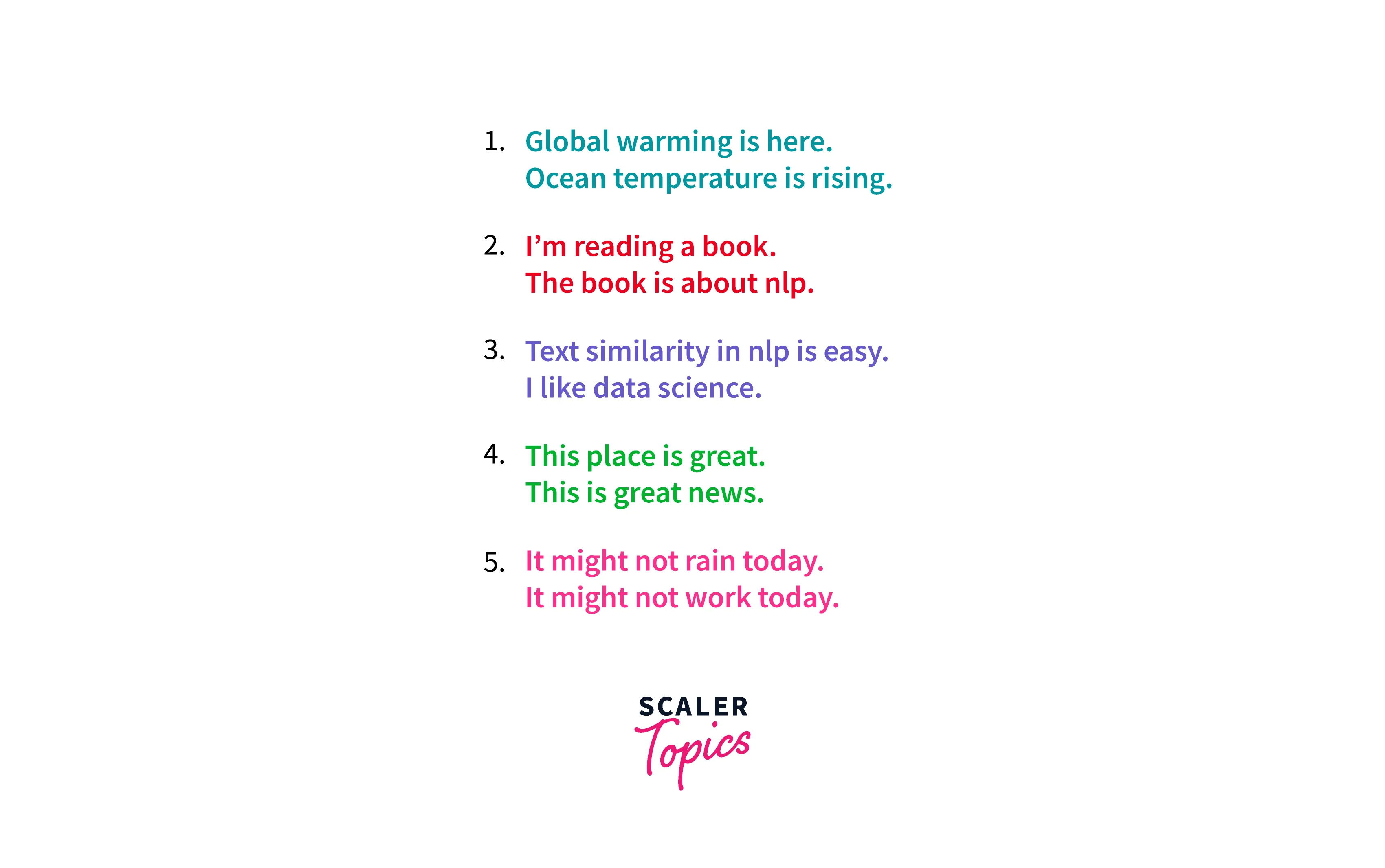
When you look at the first two pairs of sentences, you must be confident that they are similar or related in some sense. But when it comes to the rest of the 3 pairs, you might not be that confident. Also, if you observe, the last 3 pairs of sentences are not related in any way at all and cannot be called similar sentence pairs like the first two.
Surprisingly though, for models in natural language processing, it is the opposite. According to the working of text similarity in NLP, the first two pairs of sentences are not similar. However, the last two are! How? We'll find out the methods for finding text similarity in NLP soon. Let's address a couple of other things first.
Scaler Placement Report and Statistics
Scaler learners achieved 2.5x salary growth with average post-Scaler CTC reaching ₹23L.
The Similarity Problem
What is the problem that we are trying to address here? We are trying to find text similarity using NLP or just some similarity between texts. To find this, we must first define two aspects.
- The method that will be used to calculate the similarities.
- The algorithm that will be used for the transformation of our texts to embeddings.
Embeddings are just how texts are represented in the vector space.
Transform Your Career
Choose from our industry-leading programs designed for career success
Modern Software and AI Engineering Program
Master full-stack development with AI integration

Modern Data Science and ML with specialisation in AI
Advanced data science techniques with AI specialization
Advanced AIML with Specialisation in Agentic AI
Deep dive into AIML with focus on Agentic systems
DevOps, Cloud & AI Platform Engineering
Build and manage AI-powered cloud infrastructure
AI Engineering Advanced Certification by IIT-Roorkee
Premier AI engineering certification from IIT-Roorkee
Pre-processing for Text Similarity
Now, before we get started with the two aspects discussed above, we must first pre-process our text to find out text similarity using NLP. The pipeline that we are going to use for pre-processing is - Normalization, Tokenization, Removal of Stop Words, Stemming & Lemmatization.
For this pre-processing pipeline, we will make use of one of the most popular libraries in python - NLTK. Here's the code for the same.
Once all this preprocessing is done, the next task in hand is to decide the algorithm that we would use to convert our processed text into embeddings. A few of the algorithms that can be used are:
TF-IDF
TF-IDF is one of the methods that can be used to convert text to embeddings. It is short for Term Frequency - Inverse Document Frequency. Before moving on to the concept of TF-IDF, let's discuss a very basic document-term matrix.
To build a document-term matrix you only need a matrix where each row is a phrase/sentence or in NLP terms - a document and every column is a word. The values filled in the matrix are the number of times a word (column) appeared in that document (row).
Hence, the document term matrix for our 5th pair of sentences would look like this:
| DTM | it | might | not | rain | work | today |
|---|---|---|---|---|---|---|
| Doc1 | 1 | 1 | 1 | 1 | 0 | 1 |
| Doc2 | 1 | 1 | 1 | 0 | 1 | 1 |
Now, using this document term matrix, to find similarity between two documents, all you have to do is choose a similarity method and apply it to the rows of the phrases. Here's the problem with this method - every word in the phrase is given the same importance. In the two sentences above, the words that differentiate the sentences are - rain and work. These two words should be given the most importance, however, this method gives every word the same importance.
To solve this problem, we have the TF-IDF method. It also reflects the importance of a word in a document. We can get the TF-IDF importance score by getting a term's frequency (TF) and then multiplying it with the inverse document frequency (IDF). A higher importance score signifies a rare term, and hence it has higher importance. How to calculate the TF-IDF score?
Term frequency is simply the count of occurrences of the term in the document, and the inverse document frequency is calculated using the formula - . Here, dfi is the number of documents that contain the term i.
Let's look at 2 more techniques to convert text to embeddings before finding text similarity.
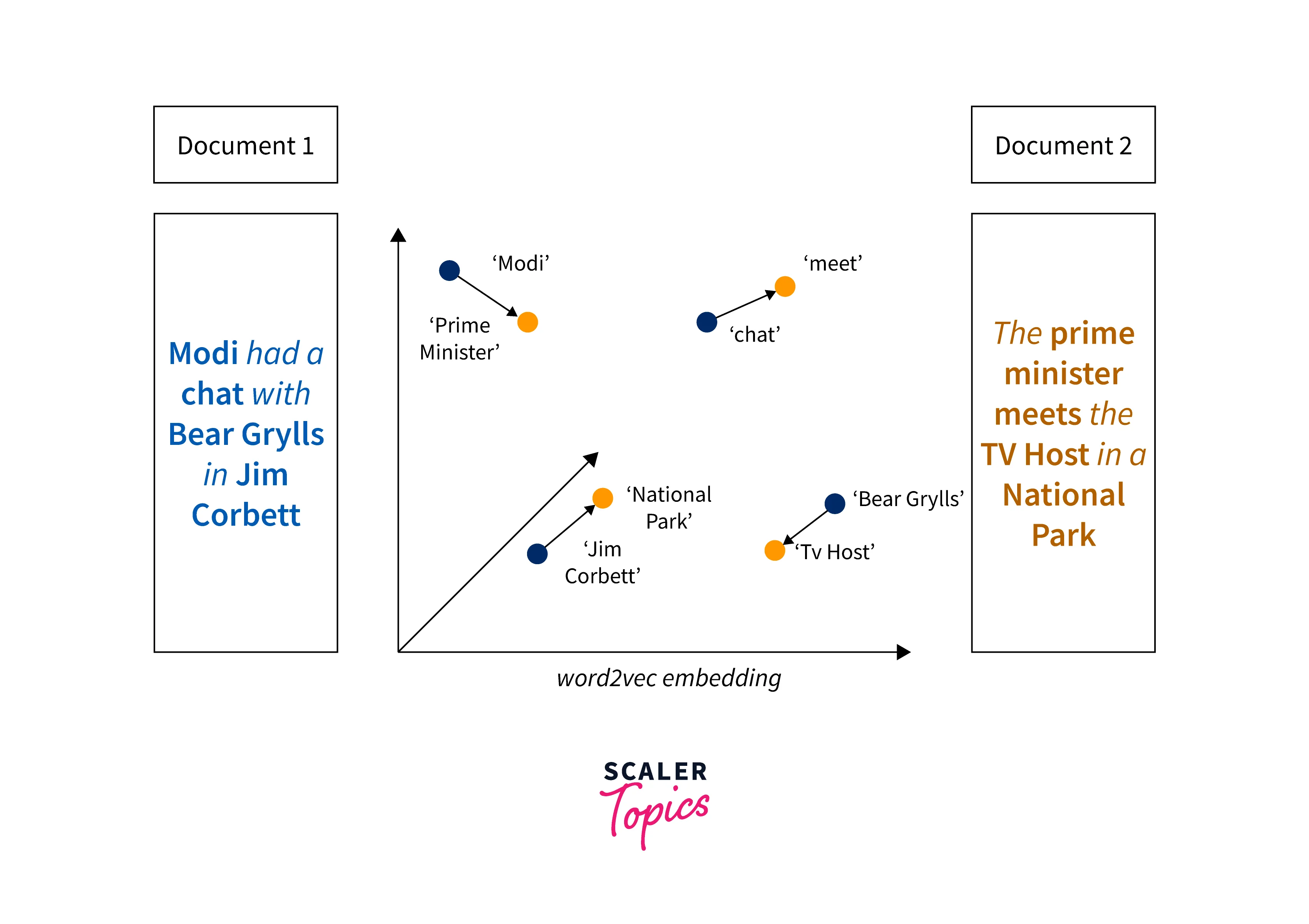
Word2Vec
This technique makes use of neural networks to represent our documents as embeddings. The Word2Vec model usually also captures the contextual meaning of words very well. The embeddings are represented as multidimensional arrays. To generate the word embeddings using Word2Vec, there are two unsupervised algorithms - Skip Gram or Continuous Bag of Words (CBOW). Both of these algorithms are architectures that make use of neural networks to learn the underlying word representations.
Continuous Bag of Words (CBOW)
In this model, the distributed representations of context, or in simpler terms, the surrounding words are combined to predict the word that lies in the middle.
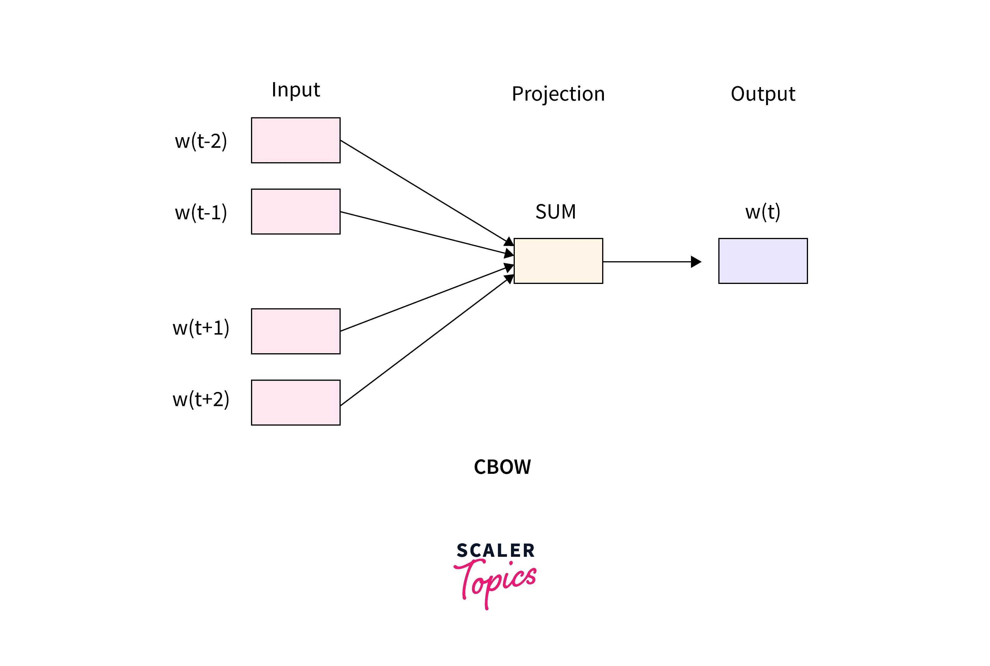
For example, if we had a sentence - "I like to drink coffee the whole day", here's what the inputs and outputs of the cbow model would look like -
| Input (Context) | Output (Target) |
|---|---|
| (I, to) | like |
| (like, drink) | to |
| (to, coffee) | drink |
| (drink, the) | coffee |
| (coffee, whole) | the |
| (the, day) | whole |
| (whole) | day |
Skip-Gram
The Skip-Gram model is the complete opposite of the continuous bag of words (CBOW) model. Here, instead of using the surrounding words to predict the middle word, we pass as input a target word to predict the neighboring words.
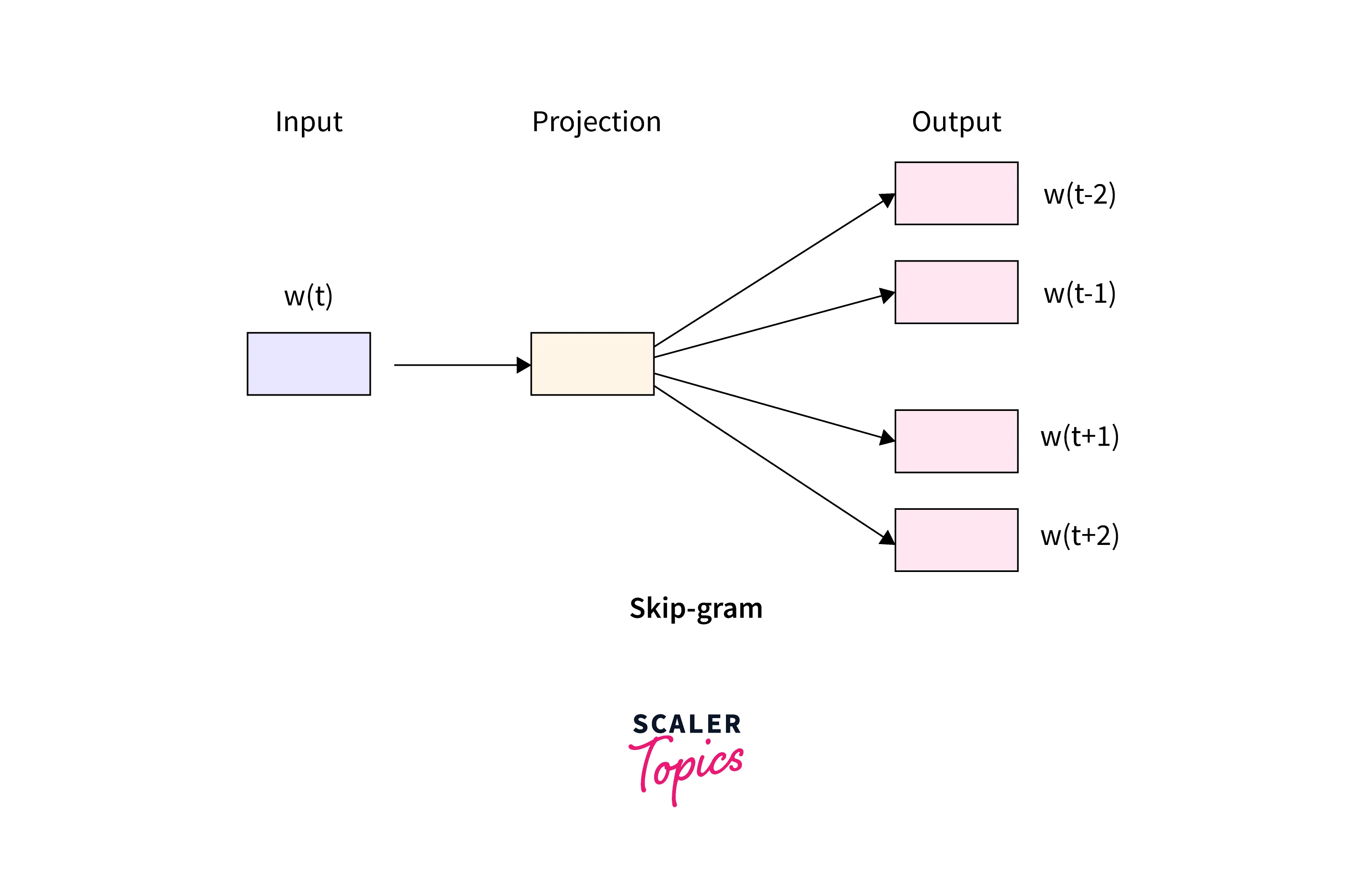
For the same sentence as above, the inputs and outputs of the skip-gram model would look like this -
| Input | Output |
|---|---|
| like | (I, to) |
| to | (like, drink) |
| drink | (to, coffee) |
| coffee | (drink, the) |
| the | (coffee, whole) |
| whole | (the, day) |
| day | (whole) |
Methods to Find Text Similarity in NLP
Now that we have discussed some algorithms that can be used to convert the text into embeddings, we can move on to the second aspect -- the statistical method that will be used to compute similarities.
Turn Learning into Career Growth
Cosine Similarity
Cosine similarity is most definitely the most widely used method to compare vectors. In simple terms, cosine similarity is just the dot product between two vectors or the cosine angle between two vectors.
To find the dot product between two vectors A and B, we use the formula:
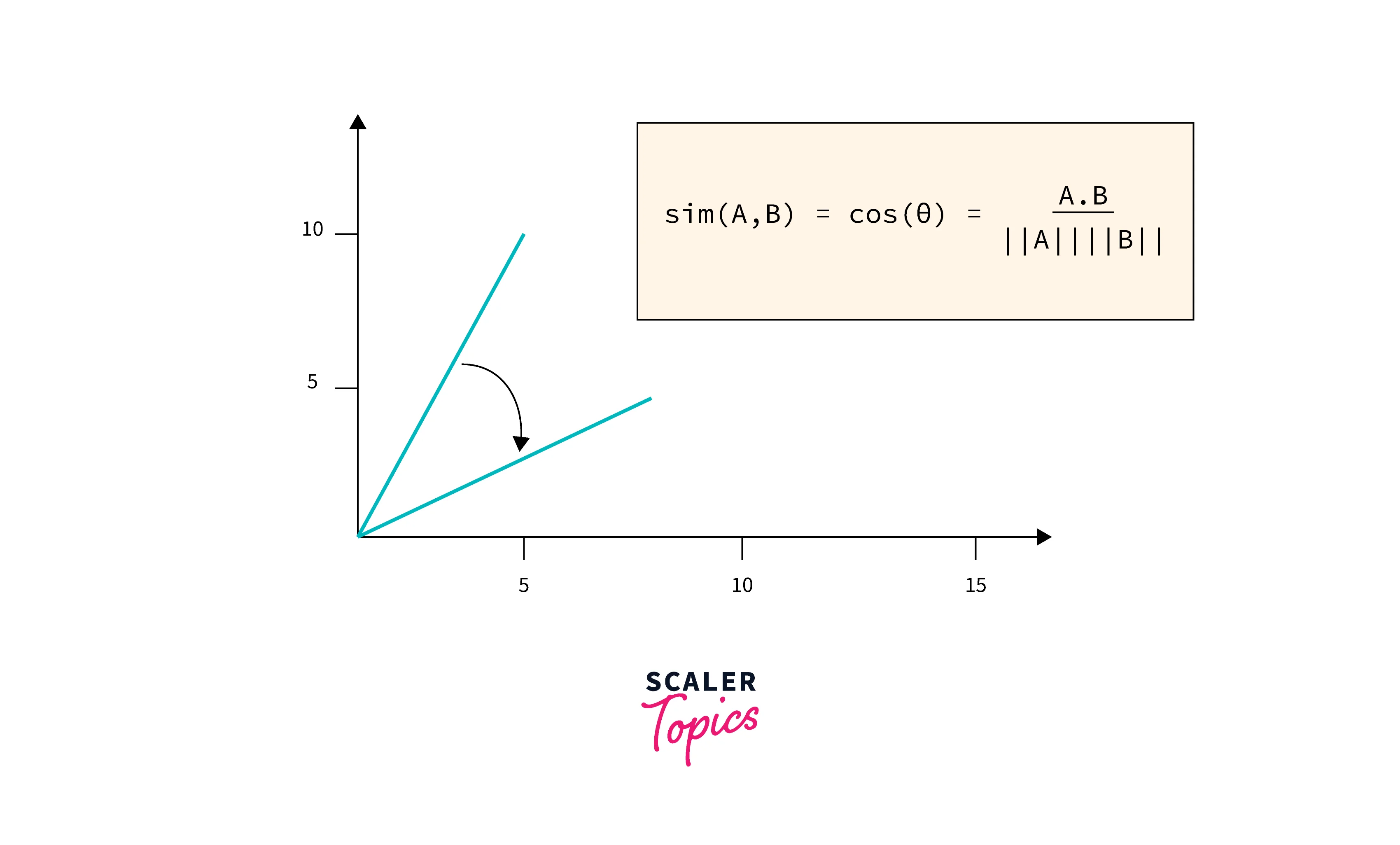
Here, is the dot product of the vectors A and B which can be calculated as:
The value (length of vector ) and (length of vector ) can be calculated as:
and the same for vector B.
Example
To use cosine similarity in Python, you can import the sklearn module for the task.
Output:
Cosine similarity gives us as output the cos of an angle between 0 to 90 degrees.
- If (or ), then the 2 vectors are dissimilar.
- If (or ), then the two vectors overlap and are completely similar.
The output - 1 above signifies that the two vectors are not very similar, and not very different either. For the second output, since vec3 has almost all same values as vec1, we can see that the cosine similarity is high - 0.9983, signifying that the two vectors are extremely similar.
Euclidean Distance
Moving on to another similarity metric - Euclidean Distance. This is a simple metric that measures the distance between two points by making use of the Pythagorean theorem. To calculate the Euclidean distance between two vectors, simply apply the following formula to the calculated document vectors:
for n vectors.
Example
Let's say you have two vectors vec1 and vec2, let's find the Euclidean distance between them, mathematically, using the above formula.
vec1 = [1, 3, 2] vec2 = [5, 0, -3]
Using the above formula,
Distance =
Distance =
To implement the same in code:
Output:
Word Mover’s Distance
In both the similarity metrics discussed above, we did not take into consideration semantics. The Word Mover's distance tries to measure the semantic distance between two documents. The Word Mover's Distance leverages the results obtained from other advanced word embedding techniques such as Glove and word2vec to generate its embeddings that can be scaled to very large data sets. With these embedding techniques, we can preserve semantic relationships.
The word mover's distance between two text documents is calculated by the minimum cumulative distance that words from text document A need to travel to match exactly the point cloud of text document B.
A couple of intriguing properties of word mover's distance are:
- It does not have any hyper-parameters and is pretty straightforward to understand and use!
- It is quite comprehensible since the distance between documents may be taken down and explained as the sparse distance between a couple of individual words.
- The knowledge encoded in word2vec and glove is naturally incorporated which leads to high accuracy.
Let's now look at an example with code implementation of the word mover's distance.
Example
To use the word mover's distance, we would require some word embeddings. For the sake of this example, let's use a pre-trained word2vec embedding - the GoogleNews-vetors-negative300.bin.gz.
Now let's write down two similar sentences:
Next, we need to remove the stopwords as part of the pre-processing. We can use nltk for the same
Post this. We can make use of the gensim module for calculating the word mover's distance.
Output:
We can see that for similar sentences, the model gives us a lower distance value, and for a different sentence, we get a higher value.
Advance Techniques Overview
Let's also look at two advanced techniques for text similarity in NLP. If you're a beginner in NLP, you may choose to skip this section!
BERT
BERT, as we know, has the capability of being able to embed the essence of words inside vectors that are densely bound.
These densely bound vectors or dense vectors are called so because every value inside the vector has a value and purpose of holding that value (contradictory to sparse vectors). BERT generates these dense vectors and every encoder layer gives as output a collection of these dense vectors.
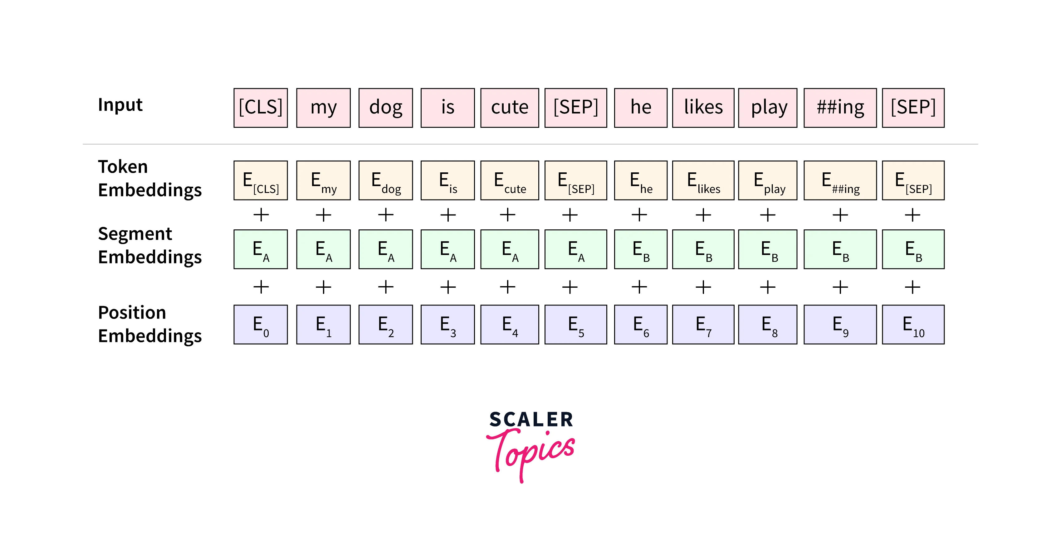
BERT essentially consists of two pre-training steps that are - Masked Language Modeling (MLM) and Next Sentence Prediction (NSP). The training text here is represented with the use of 3 embeddings -- Token Embeddings, Segment Embeddings, and Position Embeddings.
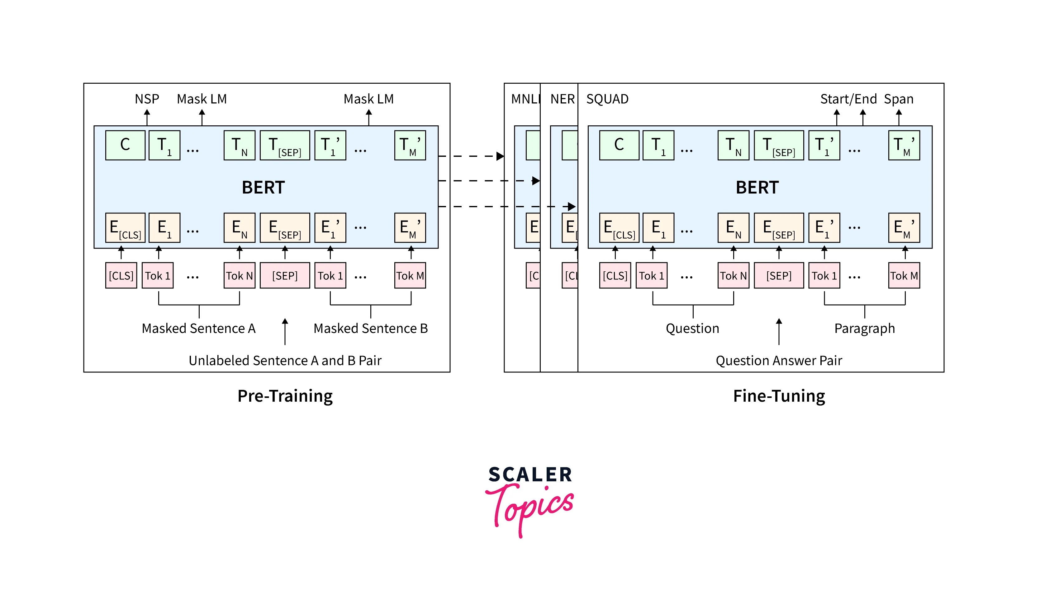
To create those "dense vectors" using BERT (embedding the corpus) we can make use of a pre-trained BERT model provided by HuggingFace. We will load the BERT base model which consists of 12 layers (transformer blocks). 110 million parameters, 12 attention heads, and a hidden size of 768.
This hidden size is essentially a vector comprising of 768 digits, and they hold a mathematical representation of a particular token (consider it as a contextual message embedding).
Implementation:
Here, after creating the embeddings using BERT, we can use cosine similarity and euclidian distances to calculate pairwise similarities and interpret the results.
Conclusion
- The problem discussed in the article is the text similarity problem in NLP. To find similarity, we define 2 aspects:
- Method of embedding
- Method to calculate similarities
- We first apply a pre-processing pipeline to our text, which would look like - Normalization, Tokenization, Removal of Stop Words, Stemming & Lemmatization.
- A few of the text embedding methods are:
- TF-IDF
- Word2Vec
- BERT
- Doc2Vec
- The 3 methods to find text similarity in NLP discussed here are:
- Cosine Similarity
- Euclidean distance
- Word Mover's distance