Transformers Optimization

Need for Transformers Optimization

Transformers optimization is essential to unlock the full potential of transformer models, enabling them to be more efficient, scalable, and effective in various NLP applications.

There are several reasons why optimizing transformers is necessary:

1. Improved Performance: Transformers Optimization techniques can help improve the performance of transformer models by reducing training time and inference latency. By optimizing the architecture, hyperparameters, and training process, transformers can achieve better accuracy and faster convergence.
2. Resource Efficiency: Transformers can require a significant amount of computational resources, including memory and processing power. Optimizing transformers can help reduce these resource requirements, making them more accessible and cost-effective.
3. Low-Resource Conditions: Optimizing transformers is particularly important in low-resource conditions, where computational resources, training data, or labeled examples are limited. Techniques such as transfer learning, data augmentation, and regularization can help improve the performance of transformers in such scenarios.
4. Model Size Reduction: Transformers can have a large number of parameters, making them memory-intensive and challenging to deploy on resource-constrained devices. Optimization techniques, such as pruning, quantization, and knowledge distillation, can reduce the size of transformer models without significantly sacrificing performance.
5. Adaptation to Specific Tasks: Transformers Optimization allows transformers to be tailored to specific tasks or domains by fine-tuning the pre-trained models. By optimizing the model's architecture, input representations, or objective functions, transformers can be better suited to handle specific NLP tasks or datasets.

Different Ways to Optimise your Transformers

Optimizing transformers involves various techniques and approaches that can enhance their performance, efficiency, and resource utilization. Here are some different ways to optimize transformers:

1. Architecture Modifications: Modifying the transformer architecture can lead to improved performance and efficiency. Some techniques include:

   • Depth-wise Separable Convolutions: Instead of using standard convolutions in the self-attention mechanism, depth-wise separable convolutions can be employed to reduce computational complexity.
   • Sparse Transformers: By introducing sparsity patterns, the number of attention connections can be reduced, resulting in faster inference and reduced memory requirements.
   • Long-Range Transformers: Long-range transformers focus on handling long sequences more efficiently by utilizing techniques like kernelized self-attention or hierarchical structures.

2. Regularization Techniques: Regularization methods help prevent overfitting and improve generalization. Some common techniques used in transformer optimization include:

   • Dropout: Dropout randomly drops out a certain percentage of the attention weights during training, which encourages the model to learn more robust representations.
   • Weight Decay: Weight decay, also known as L2 regularization, applies a penalty to the model's weights during training, discouraging large weight values and preventing overfitting.
   • Early Stopping: Early stopping involves monitoring a validation metric during training and stopping the training process when the metric starts to degrade, preventing overfitting and improving generalization.

3. Learning Rate Scheduling: Optimizing the learning rate schedule can significantly impact the training process. Some common techniques include:

   • Warmup: Warmup involves gradually increasing the learning rate at the beginning of training, allowing the model to stabilize before applying higher learning rates.
   • Learning Rate Decay: Decay techniques, such as linear decay or exponential decay, gradually reduce the learning rate over time to fine-tune the model's parameters.
   • Cyclical Learning Rates: Cyclical learning rates involve cyclically varying the learning rate between a minimum and maximum value, which can help the model escape local minima and converge faster.

4. Quantization: Quantization involves reducing the precision of the model's weights and activations, thereby reducing memory requirements and improving inference speed. Techniques like fixed-point quantization or dynamic quantization can be used.

5. Knowledge Distillation: Knowledge distillation transfers the knowledge from a larger, more complex model (teacher model) to a smaller, more efficient model (student model). This technique can help reduce the model size while retaining performance.

6. Pruning: Pruning involves removing unnecessary connections or weights from the model. Techniques like magnitude pruning, structured pruning, or lottery ticket hypothesis pruning can reduce the model size and improve inference speed.

7. Transfer Learning: Transfer learning involves utilizing pre-trained transformer models and fine-tuning them on specific tasks or domains. This approach saves training time and resources while leveraging the pre-trained model's knowledge.

These are just a few examples of the many techniques available to optimize transformers. The choice of transformers optimization methods depends on the specific requirements, constraints, and characteristics of the task at hand. It is often beneficial to experiment with multiple techniques and combinations to achieve the best results.

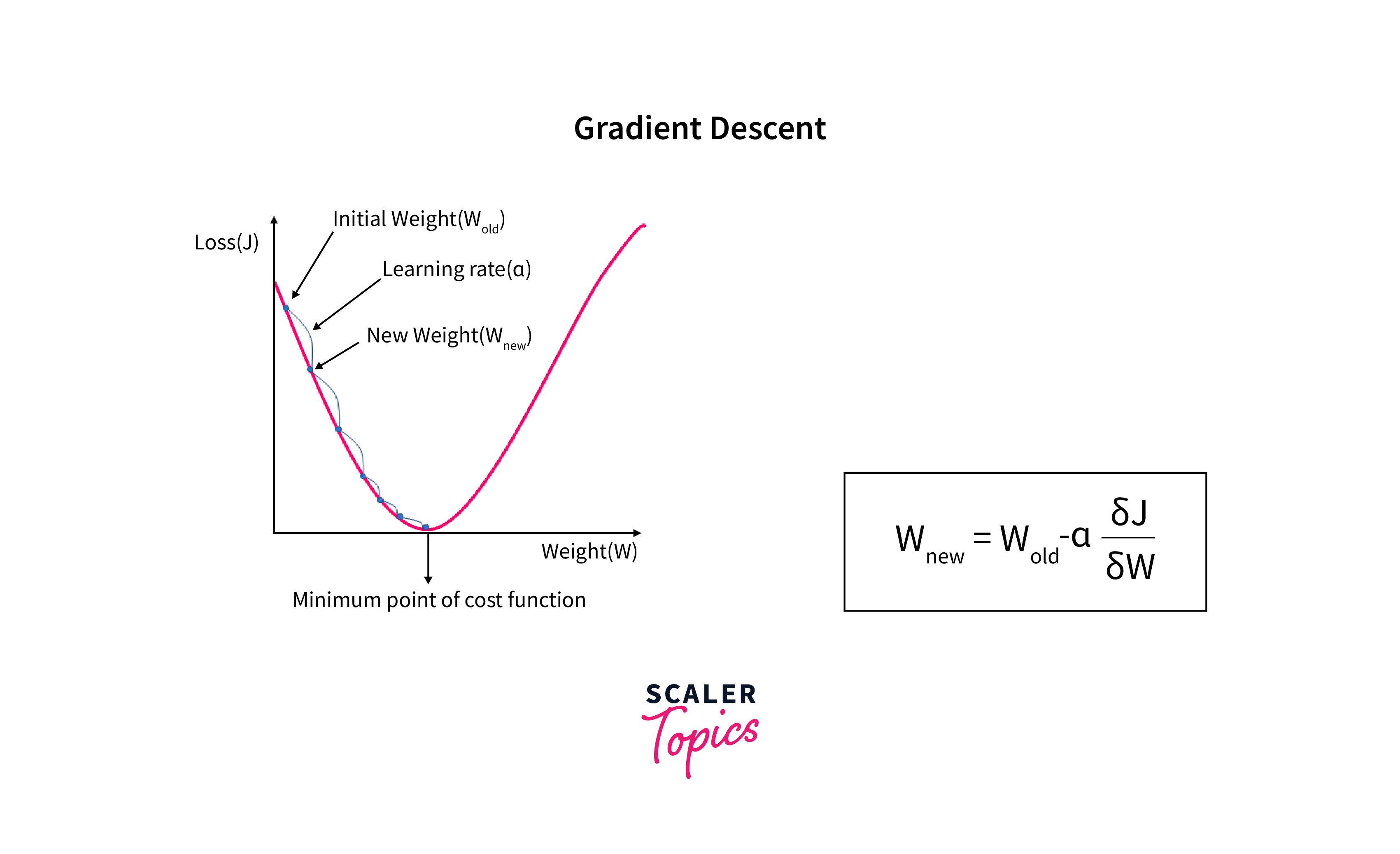
Gradient Descent and Backpropagation

In the context of Transformers, let's see Gradient Descent and Backpropagation.

• Gradient Descent: Gradient Descent is an optimization algorithm used to minimize the loss function during training. In the context of Transformers, the loss function measures how far off the model's predictions are from the actual target values. The goal is to find the model parameters (weights and biases) that minimize this loss.

• Backpropagation: Backpropagation is the algorithm used to compute gradients efficiently in neural networks, including Transformers. It works by recursively applying the chain rule of calculus to compute the gradients of the loss with respect to each layer's parameters in the network. This allows us to update the parameters using Gradient Descent.

  The chain rule can be expressed as:

  Where:

  • ∂L/∂θ is the gradient of the loss with respect to a parameter θ.
  • ∂L/∂z is the gradient of the loss with respect to the output of a layer z.
  • ∂z/∂θ is the gradient of the layer's output with respect to the parameter θ.

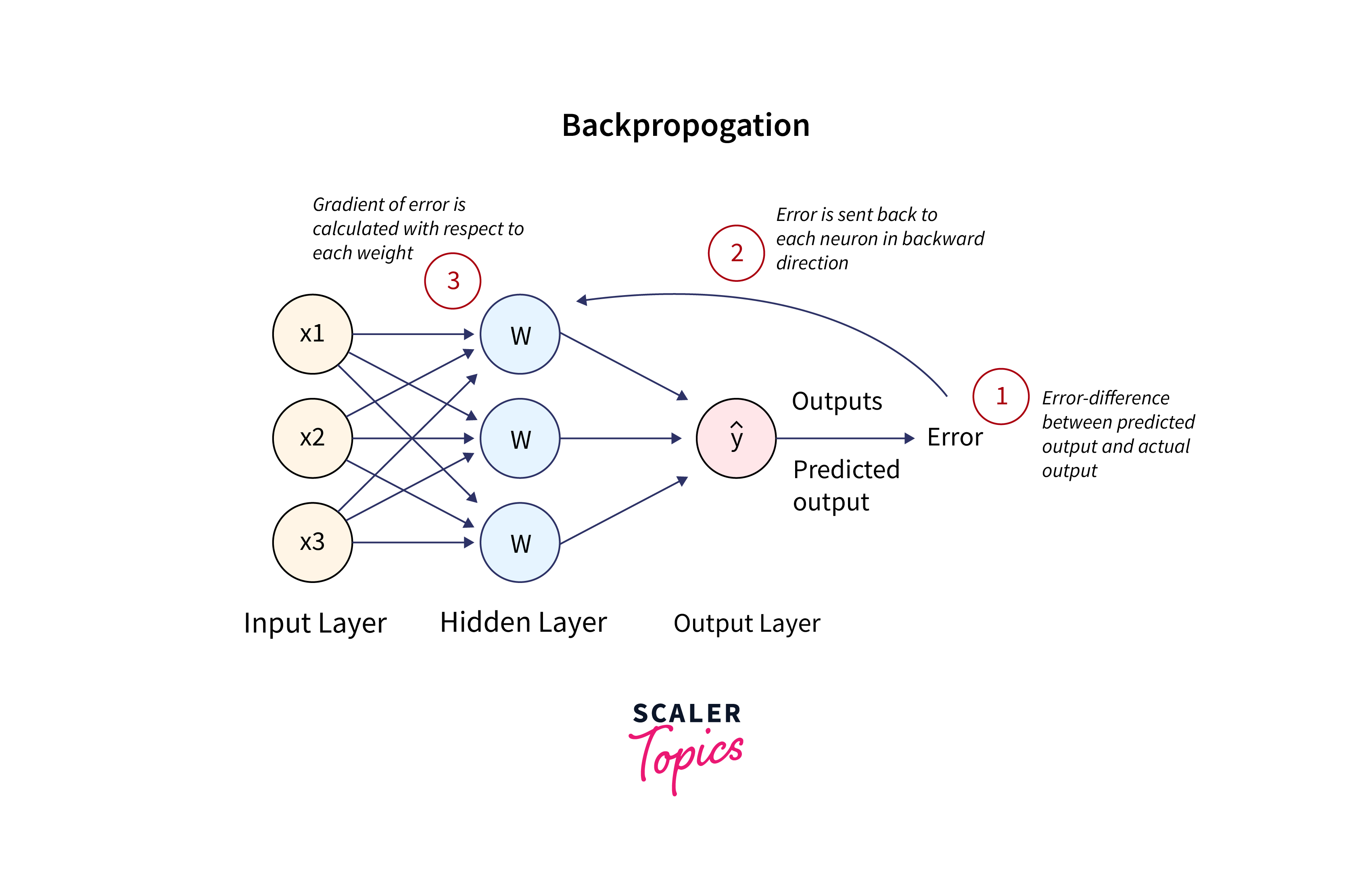
Backpropagation efficiently computes these gradients layer by layer, starting from the output layer and moving backward through the network.

Use the Hugging Face Transformers library in Python to work with pre-trained Transformers models, perform gradient descent optimization, and implement backpropagation. Here's an example of how to do this:

Output

This code demonstrates how to train a Transformers model for text classification using gradient descent and backpropagation. You can replace the example data with your own dataset and adjust hyperparameters as needed.

Adam Optimizer

Adam (short for Adaptive Moment Estimation) is an advanced optimization algorithm used in deep learning. It combines ideas from both Momentum and RMSprop to adaptively adjust the learning rates for each parameter.

• Adam maintains two moving averages: the first moment (mean) of the gradients (like momentum) and the second moment (uncentered variance) of the gradients (like RMSprop). These moving averages help control the learning rate for each parameter.
• The update rule for Adam is as follows:
  Where:
  • θ_t represents the parameters at time step t.
  • α is the learning rate.
  • β1 and β2 are exponential decay rates for the moving averages.
  • ∇L(θ_t) is the gradient of the loss with respect to θ_t.
  • ε is a small constant to prevent division by zero.

Adam adapts the learning rates for each parameter based on the magnitude of their gradients and moving averages, making it suitable for a wide range of optimization problems.

Here's an example of how to use Adam optimizer with Hugging Face Transformers:

Output

In this code, we use the AdamW optimizer from the Transformers library, which is an implementation of the Adam optimizer with weight decay (L2 regularization). You can adjust the learning rate (lr), betas, and epsilon (eps) as needed for your specific problem.

Learning Rate Scheduling

Learning Rate Scheduling is a technique used to adjust the learning rate during training. In the context of Transformers, it can be crucial for achieving faster convergence and better model performance.

• Common learning rate scheduling strategies include:
  • Step Decay: The learning rate is reduced by a fixed factor after a certain number of training steps or epochs.
  • Exponential Decay: The learning rate exponentially decreases over time.
  • Inverse Square Root Decay: The learning rate decreases proportionally to the inverse square root of the training step.
  • Warm-up and Annealing: The learning rate is gradually increased (warm-up) and then decreased (annealing) during training.
• These strategies help fine-tune the learning rate according to the training progress, allowing the model to converge more effectively and avoid overshooting the optimal parameter values.

Implement learning rate scheduling with the Hugging Face Transformers library by combining it with the PyTorch learning rate schedulers. Below is an example of how to use the torch.optim.lr_scheduler module to perform step decay learning rate scheduling during training:

Output

In this code, we define a step decay learning rate scheduler using torch.optim.lr_scheduler.StepLR. You can adjust the step_size and gamma parameters to control how often the learning rate is reduced and by what factor. This allows you to fine-tune the learning rate according to your training progress.

Weight Initialization Strategies

Weight Initialization is a crucial step in training neural networks, including Transformers. Proper initialization can help the network converge faster and achieve better performance. Here are some common weight initialization strategies:

• Zero Initialization: Setting all weights to zero is generally not recommended because it leads to symmetry issues where all neurons in a layer learn the same features and gradients become the same during backpropagation. However, it can be used in specific cases like identity mappings in residual networks.
• Random Initialization: Initializing weights with small random values is a common practice. This helps break the symmetry problem. Common methods include using Gaussian (normal) distribution or uniform distribution with appropriate scaling factors.
• Xavier/Glorot Initialization: This method sets the initial weights using a normal distribution with mean 0 and variance 2 / (fan_in + fan_out), where fan_in is the number of input units and fan_out is the number of output units. It is designed to work well with activation functions like tanh or sigmoid.
• He Initialization: Also known as the Kaiming Initialization, it is suitable for activation functions like ReLU (Rectified Linear Unit). It sets the initial weights using a normal distribution with mean 0 and variance 2 / fan_in.
• Lecun Initialization: Designed for activation functions like Leaky ReLU, it uses a normal distribution with mean 0 and variance 1 / fan_in.

Proper weight initialization can significantly impact the training dynamics of a Transformer network and prevent issues like vanishing or exploding gradients.

Here's an example of how to initialize a model with Xavier/Glorot initialization:

Output

In this code, we define a custom weight initialization function xavier_init that applies Xavier/Glorot initialization to linear (fully connected) and convolutional layers. We then use the model.apply method to apply this initialization to all layers in the model.

Regularization Techniques

Regularization is used to prevent overfitting, where a model learns to fit the training data too closely and performs poorly on unseen data. In the context of Transformers, common regularization techniques include:

• L2 Regularization (Weight Decay): This adds a penalty term to the loss function that discourages large weight values by adding the sum of squared weights to the loss. The loss becomes:

• Dropout: Dropout is a technique where during training, random neurons are set to zero with a certain probability (dropout rate), which helps prevent co-adaptation of neurons. It acts as a form of regularization by reducing model reliance on specific neurons.

• Layer Normalization: Similar to Batch Normalization (see below), Layer Normalization normalizes the activations of each layer. It can help with training stability and regularization.

• Weight Tying: In some Transformer variants, weights are tied between the encoder and decoder layers, which can act as a regularization method and improve generalization.

• Early Stopping: This technique involves monitoring the validation loss during training and stopping training when the loss starts to increase, indicating overfitting.

Regularization techniques help control the complexity of the Transformer model and promote better generalization to unseen data.

You can apply dropout regularization to Transformer-based models using the Hugging Face Transformers library. Here's an example of how to do it:

Output

In this code, we apply dropout regularization by modifying the model.dropout attribute with the desired dropout rate. You can adjust the dropout_rate parameter to control the dropout strength based on your specific needs.

Batch Normalization

Batch Normalization (BatchNorm) is a technique used to improve the training stability and speed up convergence in deep neural networks, including Transformers. It normalizes the activations of each layer across a batch of data. The normalization is applied independently to each feature (dimension) within the batch.

• The formula for BatchNorm is as follows:

  Where:

  • x is the input to the BatchNorm layer.
  • μ is the mean of x over the batch.
  • σ^2 is the variance of x over the batch.
  • γ and β are learnable scale and shift parameters.
  • ε is a small constant added for numerical stability.

• BatchNorm helps mitigate issues like internal covariate shift, enables the use of higher learning rates, and acts as a form of regularization by reducing the risk of overfitting.

In Transformers, Layer Normalization is often used instead of Batch Normalization. Here's an example of how you can add Layer Normalization to a Transformer model using Hugging Face's Transformers library: