Principal Component Analysis (PCA)

Introduction to Principal Component Analysis

Principal component analysis (PCA) is a dimensionality reduction technique to reduce the dimensionality (number of input features or columns) of a data set in which there are a large number of interrelated variables, while retaining as much as possible of the variation present in the data set.

This reduction in dimensionality is achieved by transforming the original data to a new set of variables called the principal components (PCs), which are uncorrelated and can be ordered so that the first few PCs can retain most of the variation present in all of the original variables of the dataset.

Computation of the principal components: Done by formulating the original data as a correlation or covariance matrix and computing eigenvalue-eigenvector values and then deriving new components, which are linear combinations of weights (or eigenvectors) and transformed data as PCs.

Understanding Concepts Behind PCA

Generally, most algorithms make some strict assumptions about input data, and the curse of dimensionality & multi-collinearity degrades both the training time and performance of models. In such cases finding new variables which are combinations of input variables, be it linear or non-linear, can help.

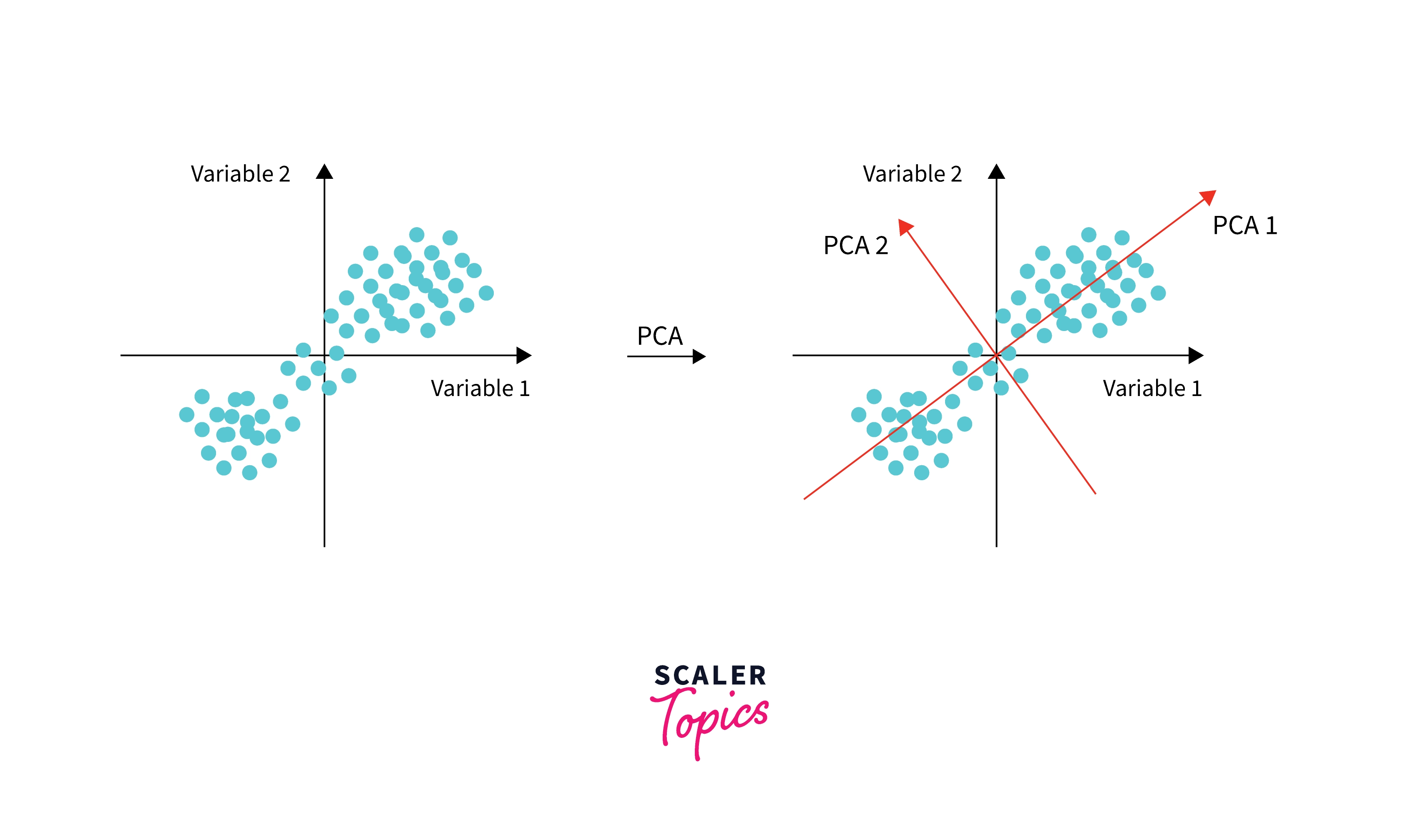
In PCA, we do this by finding lines (2D) or planes (3D) or hyper-planes(>3 dimensions), which are unit vectors (or projections) orthogonal (or perpendicular) to original features.

Objective Function of PCA

• Let us look at the objective function for the first PC1 with unit vector u1 (direction of most varying variance on the original data plane):

The objective function for PC1: We want to minimize the mean perpendicular distance from the PC line for all points.

$min(\frac{1}{n}\Sigma_i^n(x_i^Tx_i-(u_1^Tx_i)^2))$

It is proved that this function reaches a minimum when the value of u1 equals the Eigen Vector of the covariance matrix of X.

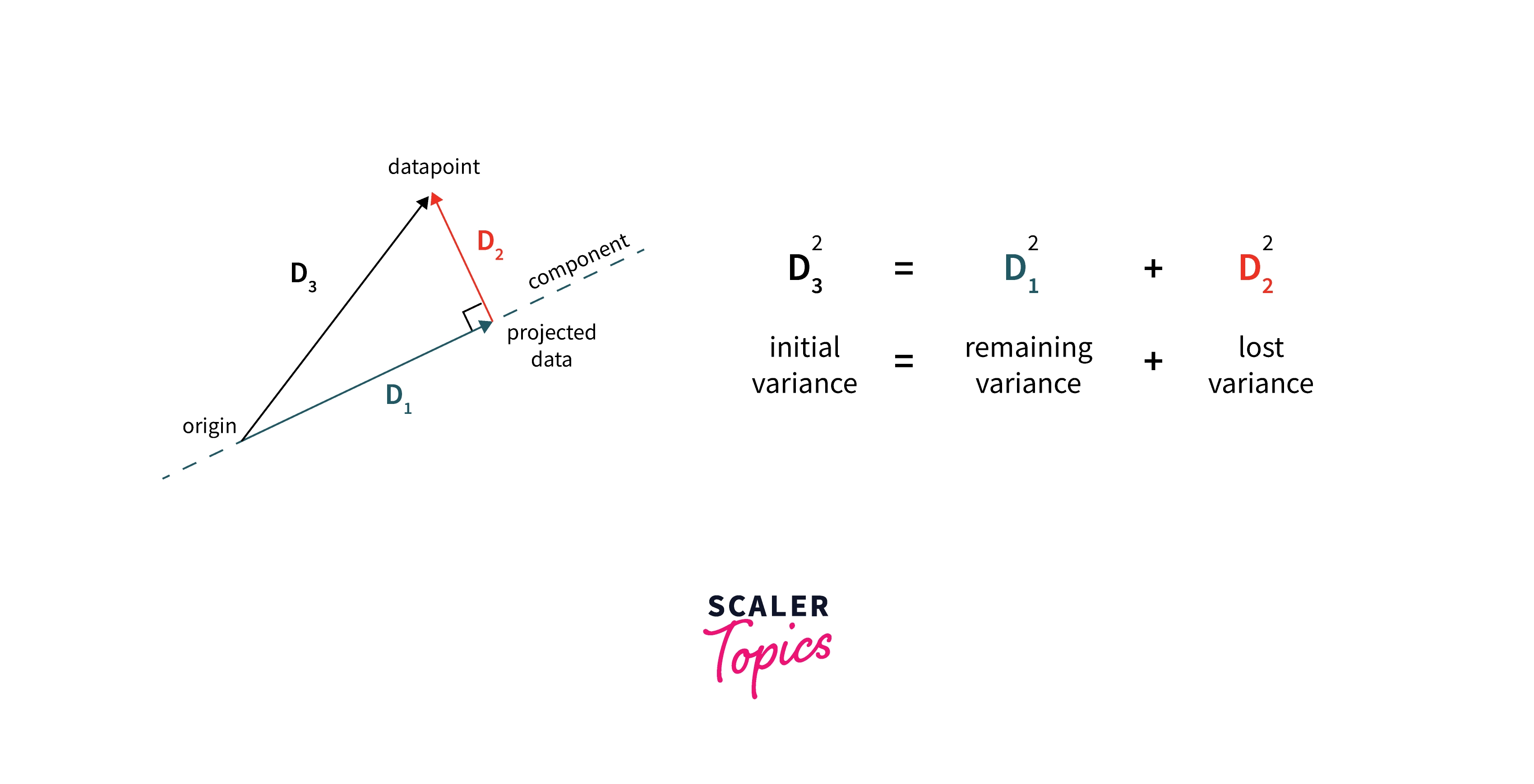
In the illustration, we can see that to maximize the variance of projections (or unit vector) D1. We need to minimize the lost variance in data D2 where D3 is constant. Hence we get the above objective function.

• Like this, we can find the second PC to the data, which is the next best direction to explain the remaining variance and also is perpendicular to the first PC.

We simply find all the eigenvectors, which are as many columns in the dataset, and they are all orthogonal to each other and explain the maximum variance in the dataset.

Mean, Std Deviation, Variance

• Mean is a measure of central tendency giving an idea of the central value of distribution.
• Standard deviation (SD) is a measure of dispersion that gives the spread of distribution around the mean.
• Variance is another measure of how far the data set variable is spread out, like SD. It is mathematically defined as the average of the squared differences (SD) from the mean of a random variable(X).
• Covariance is a measure of how two variables are related to each other - If two variables are moving in the same direction with respect to each other or not.
• Correlation is another way of looking at relationship between two variables like covariance, which is normalized to 0 to 1 scale.

What is an Eigen Value and Eigen Vector

• Multiplying an n×n matrix A (with real elements) with n-dimensional vector x:
  • Produces a matrix-vector product Ax which is well-defined and whose output is again an n-dimensional vector.
  • Generally changes the direction of the output.
• There are some special vectors that don't change the direction of the non-zero input vector.
  • Multiplication by the matrix A only stretches or contracts or reverses vector x, but it does not change its direction.

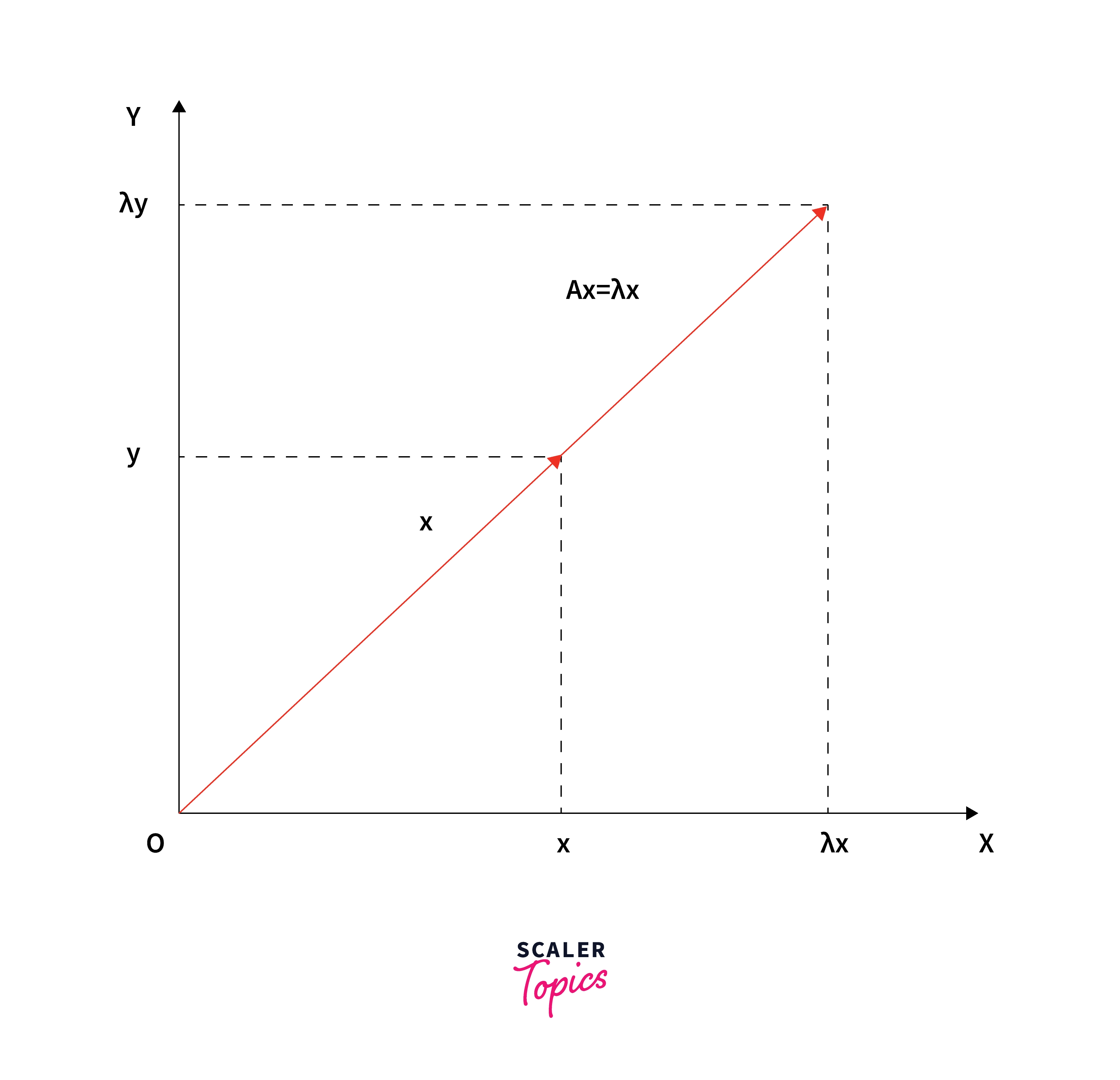
These special vectors and their corresponding values λ’s are called eigenvectors and eigenvalues of the original matrix - A: Ax = λx.

Steps to Compute Principal Components from Scratch

We will look at steps to compute the principal components here, which will also tell us how the actual principal components in the algorithm are getting derived.

To perform PCA from scratch, we follow the below steps:

• Import the data and standardize the data
• We then compute the Covariance Matrix on the input dataset.
• We then derive the corresponding eigenvalues and Eigen Vectors on the normalized dataset
• We can then finally get the Principal Component Features by taking dot product of eigenvector and standardized columns.

How many principal components should one keep? Typically after performing PCA, we can sort the eigenvalue and normalize them and look at the top few components - typically, top x components cover more than y% of variance (x~ 2 to 5, y~90).

Properties of Principal Components

When learning about what PCA is, it is important to understand the properties of PCs:

• The principal components are linear combinations of the original features.
• The principal components are also orthogonal - the correlation between any pair of these PCs is zero.
• The importance of each principal component decreases when going from 1 to n when sorted by their eigenvalues - first PC has the most importance and the last PC will have the least importance.
• The number of these PCs is either equal to or less (by design) than the original features present in the dataset after performing the feature selection with PCA.

Data Treatment for Conducting PCA

• We should normalize the continuous variables by centering to the mean and dividing by standard deviation.
• Mixing ordinal with numerical variables is not possible in PCA due to correlation/covariance calculations and standardizing data.
• Instead we can use Categorical versions of PCA or non-linear PCA for categorical / ordinal data.

Normalization of Features

Normalization (or Z-score normalization) or standardization (or Z-score normalization) is one of the important pre-preprocessing steps for PCA. It involves rescaling the features such that they have the properties of a standard normal distribution with a mean of zero and a standard deviation of one.

If not for normalization, the components vary differently (e.g. human height vs. weight) because of their respective scales (meters vs. kilos). PCA might determine that the direction of maximal variance (objective in PCA) corresponds highest with the ‘weight’ immaterial of other features if scaling is not done.

Implementing PCA with Scikit-Learn

• Setting up the jupyter notebook Jupyter Notebook can be installed from the popular setup of Anaconda or jupyter directly. Reference instructions for setting up from the source can be followed from here. Once installed we can spin up an instance of the jupyter notebook server and open a python notebook instance, and run the following code for setting up basic libraries and functionalities.

If a particular library is not found, it can simply be downloaded from within the notebook by running a system command pip install sample_library command. For example, to install pandas, run the command from a cell within jupyter notebook like:

• Preprocessing: Splitting the dataset into train and test sets such that they have 80/20 splits, and then we normalize the data

• Applying PCA: Here we load the PCA algorithm from sklearn and then fit it on the training data
• We then transform the test data with the earlier pre-processing steps

Results with First 2 and First 3 Principal Components

• Training and Making Predictions: We can take the output of PCA as input to other models, here let us first try the first 2 and 3 principal components and then model with all the components and then with the full feature set
• We are loading and training an RF algorithm from sklearn and then evaluating its performance

Results with Full Feature Set

Output: of the different models:

• We can see that the results are comparably the same with the first and three components with decent accuracy when compared with a full feature set.
• One thing to note here is that this is a relatively simple and small dataset. Otherwise, on big datasets, with the first few components themselves, we can get good results without the issues of collinearity and noise.

Weights of Principal Components

The weights of PCs are the eigenvectors of the mean-centered data. We can also see that the principal components are the dot product of weights and the mean-centered data(X).

So we can use both methods to retrieve the weights.

$PC_i = Weights_i * X_{mean\space centered\space data}$

Percentage of Variance Explained With Each PC

After performing PCA, we get variance scores for each PC. These are simply the eigenvalues for each PC sorted in descending order and normalized so that they sum to 1. We can use a scree plot to visualize the cumulative variance by the number of PCs and select the appropriate number of PCs depending on the model we have further.

Plot the Clustering Tendency

Generally, while doing EDA or showing the output of any model, we can not visualize all the dimensions together with the labels in a single plot. In these cases plotting the first two dimensions along with the class labels or target value will reveal interesting patterns and insights for further understanding.

How to Get the Original Features Back

The fitted pca object has the inverse_transform method that gives back the original data when you input principal components features.

Pseudo code for inverse transform in PCA (assuming normalized data):

Advantages of PCA

• While decoding what PCA is, we can see that PCA can be used for producing derived variables from original data with decent properties, so it can be further used in many supervised learning problems like regression, clustering, etc.
• PCA also serves as a tool for data visualization of the original dataset in exploration and understanding the output of many algorithms (in the visualization of the observations or visualization of the variables).
• PCA can also be used as a tool for data imputation for filling in missing values in a data matrix.