Word Classes and Part-of-Speech Tagging in NLP

Overview

Part-of-speech (POS) tagging is an important Natural Language Processing (NLP) concept that categorizes words in the text corpus with a particular part of speech tag (e.g., Noun, Verb, Adjective, etc.)

POS tagging could be the very first task in text processing for further downstream tasks in NLP, like speech recognition, parsing, machine translation, sentiment analysis, etc.

The particular POS tag of a word can be used as a feature by various Machine Learning algorithms used in Natural Language Processing.

Introduction

Simply put, In Parts of Speech tagging for English words, we are given a text of English words we need to identify the parts of speech of each word.

Example Sentence : Learn NLP from Scaler

Learn -> ADJECTIVE NLP -> NOUN from -> PREPOSITION Scaler -> NOUN

Although it seems easy, Identifying the part of speech tags is much more complicated than simply mapping words to their part of speech tags.

Why Difficult ?

Words often have more than one POS tag. Let’s understand this by taking an easy example.

In the below sentences focus on the word “back” :

Sentence	POS tag of word “back”
The “back” door	ADJECTIVE
On my “back”	NOUN
Win the voters “back”	ADVERB
Promised to “back” the bill	VERB

The relationship of “back” with adjacent and related words in a phrase, sentence, or paragraph is changing its POS tag.

It is quite possible for a single word to have a different part of speech tag in different sentences based on different contexts. That is why it is very difficult to have a generic mapping for POS tags.

If it is difficult, then what approaches do we have?

Before discussing the tagging approaches, let us literate ourselves with the required knowledge about the words, sentences, and different types of POS tags.

Word Classes

In grammar, a part of speech or part-of-speech (POS) is known as word class or grammatical category, which is a category of words that have similar grammatical properties.

The English language has four major word classes: Nouns, Verbs, Adjectives, and Adverbs.

Commonly listed English parts of speech are nouns, verbs, adjectives, adverbs, pronouns, prepositions, conjunction, interjection, numeral, article, and determiners.

These can be further categorized into open and closed classes.

Closed Class

Closed classes are those with a relatively fixed/number of words, and we rarely add new words to these POS, such as prepositions. Closed class words are generally functional words like of, it, and, or you, which tend to be very short, occur frequently, and often have structuring uses in grammar.

Example of closed class-

Determiners: a, an, the Pronouns: she, he, I, others Prepositions: on, under, over, near, by, at, from, to, with

Open Class

Open Classes are mostly content-bearing, i.e., they refer to objects, actions, and features; it's called open classes since new words are added all the time.

By contrast, nouns and verbs, adjectives, and adverbs belong to open classes; new nouns and verbs like iPhone or to fax are continually being created or borrowed.

Example of open class-

Nouns: computer, board, peace, school Verbs: say, walk, run, belong Adjectives: clean, quick, rapid, enormous Adverbs: quickly, softly, enormously, cheerfully

Tagset

The problem is (as discussed above) many words belong to more than one word class.

And to do POS tagging, a standard set needs to be chosen. We Could pick very simple/coarse tagsets such as Noun (NN), Verb (VB), Adjective (JJ), Adverb (RB), etc.

But to make tags more dis-ambiguous, the commonly used set is finer-grained, University of Pennsylvania’s “UPenn TreeBank tagset”, having a total of 45 tags.

Tag	Description	Example	Tag	Description	Example
CC	Coordin. Conjunction	and, but, or	SYM	Symbol	+%, &
CD	Cardinal number	one, two, three	TO	"to"	to
DT	Determiner	a, the	UH	Interjection	ah, oops
EX	Existential 'there'	there	VB	Verb, base form	eat
FW	Foreign word	mea culpa	VBD	Verb, past tense	ate
IN	Preposition/sub-conj	of, in, by	VBG	Verb, gerund	eating
JJ	Adjective	yellow	VBN	Verb, past participle	eaten
JJR	Adj., comparative	bigger	VBP	Verb, non-3 sg pres	eat
JJS	Adj., superlative	wildest	VBZ	Verb, 3 sg pres	eats
LS	List item marker	1, 2, One	WDT	Wh-determiner	which, that
MD	Modal	can, should	WP	Wh-pronoun	what, who
NN	Noun, sing. or mass	llama	WP$	Possessive wh-	whose
NNS	Noun, plural	llamas	WRB	Wh-adverb	how, where
NNP	Proper noun, singular	IBM	$	Dollar sign	$
NNPS	Proper noun, plural	Carolinas	#	Pound sign	#
PDT	Predeterminer	all, both	"،	Left quote	( or )
POS	Possessive ending	's	"	Right quote	( or )
PRP	Personal pronoun	I, you, he	(	Left parenthesis	([,(,{,<)
PRP$	Possessive pronoun	your, one's	)	Right parenthesis	(],),},>)
RB	Adverb	quickly, never	,	Comma
RBR	Adverb, comparative	faster	.	Sentence-final punc	(. ! ?)
RBS	Adverb, superlative	fastest	:	Mid-sentence punc	(: ; ...)
RP	Particle	up, off

What Are Parts of Speech Tagging in NLP?

Part-of-speech tagging is the process of assigning a part of speech to each word in a text. The input is a sequence $x_1, x_2,..., x_n$ of (tokenized) words, and the output is a sequence $y_1, y_2,..., y_n$ of POS tags, each output $y_i$ corresponding exactly to one input $x_i$ .

part of speech tagger

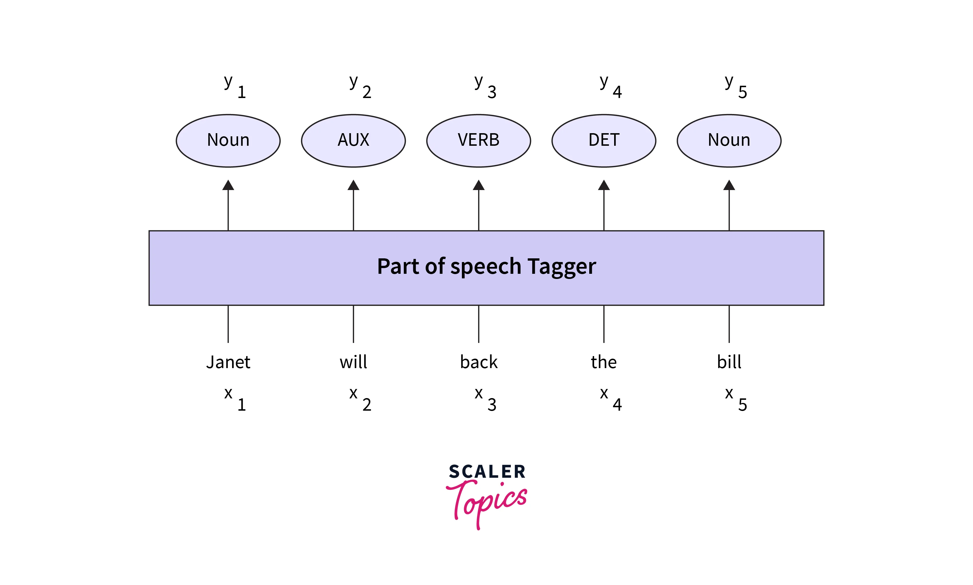
Tagging is a disambiguation task; words are ambiguous i.e. have more than one a possible part of speech, and the goal is to find the correct tag for the situation.

For example, a book can be a verb (book that flight) or a noun (hand me that book).

The goal of POS tagging is to resolve these ambiguities, choosing the proper tag for the context.

POS tagging Algorithms Accuracy:

The accuracy of existing State of the Art algorithms of part-of-speech tagging is extremely high. The accuracy can be as high as ~ 97%, which is also about the human performance on this task, at least for English.

We’ll discuss algorithms/techniques for this task in the upcoming sections, but first, let’s explore the task. Exactly how hard is it?

Let's consider one of the popular electronic collections of text samples, Brown Corpus. It is a general language corpus containing 500 samples of English, totaling roughly one million words.

In Brown Corpus :

85-86% words are unambiguous - have only 1 POS tag

but,

14-15% words are ambiguous - have 2 or more POS tags

Particularly ambiguous common words include that, back, down, put, and set.

The word back itself can have 6 different parts of speech (JJ, NN, VBP, VB, RP, RB) depending on the context.

Nonetheless, many words are easy to disambiguate because their different tags aren’t equally likely. For example, "a" can be a determiner or the letter "a", but the determiner sense is much more likely.

This idea suggests a useful baseline, i.e., given an ambiguous word, choose the tag which is most frequent in the corpus.

This is a key concept in the Frequent Class tagging approach.

Let’s explore some common baseline and more sophisticated POS tagging techniques.

Rule-Based Tagging

Rule-based tagging is the oldest tagging approach where we use contextual information to assign tags to unknown or ambiguous words.

The rule-based approach uses a dictionary to get possible tags for tagging each word. If the word has more than one possible tag, then rule-based taggers use hand-written rules to identify the correct tag.

Since rules are usually built manually, therefore they are also called Knowledge-driven taggers. We have a limited number of rules, approximately around 1000 for the English language.

One of example of a rule is as follows:

Sample Rule: If an ambiguous word “X” is preceded by a determiner and followed by a noun, tag it as an adjective;

A nice car: nice is an ADJECTIVE here.

Limitations/Disadvantages of Rule-Based Approach:

High development cost and high time complexity when applying to a large corpus of text
Defining a set of rules manually is an extremely cumbersome process and is not scalable at all

Stochastic POS Tagging

Stochastic POS Tagger uses probabilistic and statistical information from the corpus of labeled text (where we know the actual tags of words in the corpus) to assign a POS tag to each word in a sentence.

This tagger can use techniques like Word frequency measurements and Tag Sequence Probabilities. It can either use one of these approaches or a combination of both. Let’s discuss these techniques in detail.

Word Frequency Measurements

The tag encountered most frequently in the corpus is the one assigned to the ambiguous words(words having 2 or more possible POS tags).

Let’s understand this approach using some example sentences :

Ambiguous Word = “play”

Sentence 1 : I play cricket every day. POS tag of play = VERB

Sentence 2 : I want to perform a play. POS tag of play = NOUN

The word frequency method will now check the most frequently used POS tag for “play”. Let’s say this frequent POS tag happens to be VERB; then we assign the POS tag of "play” = VERB

The main drawback of this approach is that it can yield invalid sequences of tags.

Tag Sequence Probabilities

In this method, the best tag for a given word is determined by the probability that it occurs with “n” previous tags.

Simply put, assume we have a new sequence of 4 words, $w_1 ~w_2~ w_3 ~w_4$ And we need to identify the POS tag of $w_4$ .

If n = 3, we will consider the POS tags of 3 words prior to w4 in the labeled corpus of text

Let’s say the POS tags for

$w_1$ = NOUN, $w_2$ = VERB , $w_3$ = DETERMINER

In short, N, V, D: NVD

Then in the labeled corpus of text, we will search for this NVD sequence.

Let’s say we found 100 such NVD sequences. Out of these -

10 sequences have the POS of the next word is NOUN 90 sequences have the POS of the next word is VERB

Then the POS of the word $w_4$ = VERB

The main drawback of this technique is that sometimes the predicted sequence is not Grammatically correct.

Now let’s discuss some properties and limitations of the Stochastic tagging approach :

This POS tagging is based on the probability of the tag occurring (either solo or in sequence)
It requires labeled corpus, also called training data in the Machine Learning lingo
There would be no probability for the words that don’t exist in the training data
It uses a different testing corpus (unseen text) other than the training corpus
It is the simplest POS tagging because it chooses the most frequent tags associated with a word in the training corpus

Transformation-Based Learning Tagger: TBL

Transformation-based tagging is the combination of Rule-based & stochastic tagging methodologies.

In Layman's terms;

The algorithm keeps on searching for the new best set of rules given input as labeled corpus until its accuracy saturates the labeled corpus.

Algorithm takes following Input:

a tagged corpus
a dictionary of words with the most frequent tags

Output : Sequence of transformation rules

Example of sample rule learned by this algorithm:

Rule : Change Noun(NN) to Verb(VB) when previous tag is To(TO)

E.g.: race has the following probabilities in the Brown corpus -

Probability of tag is NOUN given word is race P(NN | race) = 98%
Probability of tag is VERB given word is race P(VB | race) = 0.02

Given sequence: is expected to race tomorrow

First tag race with NOUN (since its probability of being NOUN is 98%)
Then apply the above rule and retag the POS of race with VERB (since just the previous tag before the “race” word is TO )

The Working of the TBL Algorithm

Step 1: Label every word with the most likely tag via lookup from the input dictionary.

Step 2: Check every possible transformation & select one which most improves tagging accuracy.

Similar to the above sample rule, other possible (maybe worst transformations) rules could be -

Change Noun(NN) to Determiner(DT) when previous tag is To(TO)
Change Noun(NN) to Adverb(RB) when previous tag is To(TO)
Change Noun(NN) to Adjective(JJ) when previous tag is To(TO)
etc…..

Step 3: Re-tag corpus by applying all possible transformation rules

Repeat Step 1,2,3 as many times as needed until accuracy saturates or you reach some predefined accuracy cutoff.

Advantages and Drawbacks of the TBL Algorithm

Advantages

We can learn a small set of simple rules, and these rules are decent enough for basic POS tagging
Development, as well as debugging, is very easy in TBL because the learned rules are easy to understand
Complexity in tagging is reduced because, in TBL, there is a cross-connection between machine-learned and human-generated rules

Drawbacks

Despite being a simple and somewhat effective approach to POS tagging, TBL has major disadvantages.

TBL algorithm training/learning time complexity is very high, and time increases multi-fold when corpus size increases
TBL does not provide tag probabilities

Hidden Markov Model POS Tagging: HMM

HMM is a probabilistic sequence model, i.e., for POS tagging a given sequence of words, it computes a probability distribution over possible sequences of POS labels and chooses the best label sequence.

This makes HMM model a good and reliable probabilistic approach to finding POS tags for the sequence of words.

We’ll explore the important aspects of HMM in this section; we’ll see a few mathematical equations in an easily understandable manner.

Motivation:

Before diving deep into the HMM model concepts let’s first understand the elementary First Order Markov Model (or Markov Chain) with real-life examples.

Assume we have three types of weather conditions: sunny, rainy, and foggy.

The problem at hand is to predict the next day’s weather using the previous day's weather.

Let q_n = variable denoting the weather on the n^thday

We want to find the probability of q_n given weather conditions of previous {n-1} days. This can be mathematically written as :

$P(q_n | q_{n-1}, q_{n-2} ,............., q_1) = ?$

According to first-order Markov Assumption -

The weather condition on the nth day is only dependent on the weather of (n-1)th day.

i.e. tomorrow’s weather is only dependent on today's weather conditions only.

So the above equation boils down to the following:

$P(q_n | q_{n-1}, q_{n-2} ,............., q_1) = P(q_n | q_{n-1})$

Consider the example below for probability computation :

example for probability computation

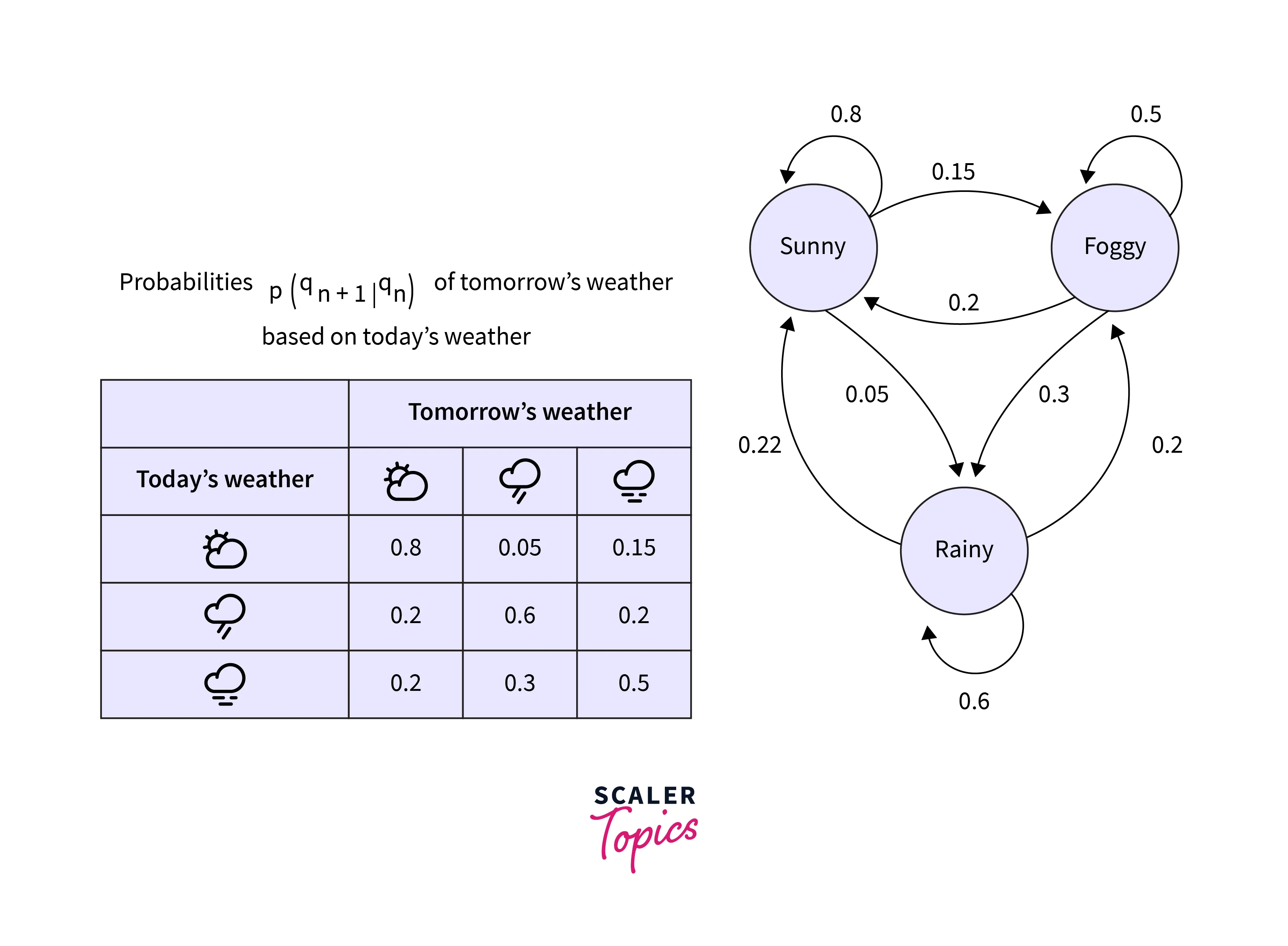
E.g.

P(Tomorrow’s weather = “Rainy” | Today’s weather = “Sunny”) = 0.05

P(Tomorrow’s weather = “Rainy” | Today’s weather = “Rainy”) = 0.6

Etc.

Let's solve a simple Question ?

Given that today’s weather is sunny, what is the probability that tomorrow will be sunny and the day after will be rainy? Mathematically $P(q_2 = sunny, q_3 = rainy | q_1 = sunny)$ ?

Let’s do simple calculations :

$P(q_2 = sunny, q_3 = rainy | q_1 = sunny)$

$= P(q_3 = rainy | q_2 = sunny, q_1 = sunny) × P(q_2 = sunny | q_1 = sunny)$

{using first-order Markov Assumption} = $P(q_3 = rainy | q_2 = sunny) × P(q_2 = sunny | q_1 = sunny)$

$= 0.05 × 0.8$

$= 0.04$

Hidden Markov Model

A Markov chain is useful when we need to compute a probability for a sequence of observable events.

In many cases, the events we are interested in are hidden, i.e., we don’t observe them directly.

For example, we don’t normally observe part-of-speech tags in a text. Rather, we see words and must infer the tags from the word sequence. We call the tags hidden because they are not observed.

A hidden Markov model (HMM) allows us to talk about both observed events (like words that we see in the input) and hidden events (like part-of-speech tags).

Simply in HMM, we consider the following;

Words : Observed POS tags : Hidden

HMM is a Probabilistic model; we find the most likely sequence of tags T for a sequence of words W

$W = w_1. . . . . w_n --------words in the sequence (observed)$ $T = t_1. . . . .t_n ---------- the corresponding POS tags (hidden/unknown)$

Objective of HMM:

We want to find out the probabilities of possible tag sequences given word sequences.

i.e. P(T | W )

And select the tag sequence that has the highest probability

Mathematically we write it like this;

$argmax_T~ P~(~T~ |~ W~ )$

Using the Bayes Theorem;

$P(T | W )$ can be written as :

$P(T | W ) = P(W | T) * P(T) / P(W)$

P(W) : Probability of Word sequence remain same

So we can just approximate** P(T | W)** as :

$P~(~T~ |~ W~ )~ =~ P~(~W~ |~ T~)~ *~ P~(~T~)$

We have already stated that W and T are word and tag sequences. Therefore we can write the above equation as follows:

$P(T | W ) = P(w_1> . . . . . w_n | t_1 . . . . . t_n) * P(t_1> . . . . . t_n) - - - - - {main~ equation}$

Let’s break down the component of this main equation.

First Part of Main Equation

$P(w_1 . . . . . w_n | t_1 . . . . . t_n) = P(w | t_1 . . . . . t_n) * P(w_2 | t_1 . . . . . t_n)................ P(w_n | t_1 . . . . . t_n)$

Using the first-order Markov assumption, The probability of a word appearing depends only on its own POS tag.

$P(w_1 | t_1 . . . . . t_n) = P(w_1 | t_1$

Therefore;

$P(w_1 . . . . . w_n | t_1 . . . . . t_n) = P(w_1 | t_1) * P(w_2 | t_2) * ................ * P(w_n | t_n)$

$P(w_1 . . . . . w_n | t_1 . . . . . t_n) =* \prod_{i=1}^{n}*P(w_i | t_i)$

Second Part of Main Equation

$P(t_1 . . . . . t_n) = ?$

The probability of a tag is dependent only on the previous tag rather than the entire tag sequence - Also called Bigram assumption

$P(t_1 . . . . . t_n) =* \prod_{i=1}^{n}*P(t_i | t_{i-1} )$

Therefore the main equation becomes :

$P(T | W) =* \prod_{i=1}^{n}*P(w_i | t_i )* \prod_{i=1}^{n}*P(t_i | t_{i-1} )$

For possible POS tag sequences (T), we compute this probability and consider that tag sequence that gives the maximum value of quantity.

Here,

$\prod_{i=1}^{n}P(w_1 | t_i</sub> )$ : Word likelihood probabilities or emission probability

$\prod_{i=1}^{n}P(t_i | t_{i-1} )$ : Tag Transition probabilities

The computation of the above probabilities requires a dynamic programming approach, and the algorithm is called The Viterbi Algorithm. Understanding the Viterbi algorithm requires another article in itself.

Below is a simple example of the computation of Word likelihood probabilities and Tag Transition probabilities from the Brown corpus -

Tag Transition probabilities $p\left(t_i \mid t_{i-1}\right)$

\begin{gathered} P\left(t_i \mid t_{i-1}\right)=\frac{C\left(t_{i-1}, t_i\right)}{C\left(t_{i-1}\right)} \\ P(N N \mid D T)=\frac{C(D T, N N)}{C(D T)}=\frac{56,509}{116,454}=0.49 \end{gathered}

Word Likelihood probabilities $p\left(w_i \mid t_i\right)$

\begin{gathered} P\left(w_i \mid t_i\right)=\frac{C\left(t_i, w_i\right)}{C\left(t_i\right)} \\ P(i s \mid V B Z)=\frac{C(V B Z, i s)}{C(V B Z)}=\frac{10,073}{21,627}=0.47 \end{gathered}

Tagging Unknown Words

It is very much possible that we encounter new/unseen words while tagging sentences/sequences of words. All of the approaches/algorithms discussed above will fail if this happens. For example, on average new words are added to newspapers/language 20+ per month.

Few Hacks/Techniques to Tackle New Words:

Assume they are nouns (most of the new words we see falls into the NOUN (NN) POS
Use capitalisation, suffixes, etc. This works very well for morphologically complex
We could look at the new word's internal structure, such as assigning NOUNS (NNS) for words ending in 's.'
For probabilistic-based models, new word probabilities are zero, and there are smoothing techniques. A naïve technique is to add a small frequency count (say 1) to all words, including unknown words

Conclusion

In this article, we discussed a very high-level overview of POS tagging a sequence of words/sentences without deep diving into too much math, technical jargon, and code.

We discussed the following in this article:

Understood what POS tagging is, why this is very useful in NLP, also why POS tagging difficult
We have understood the word classes and semantic structure of sentences and seen a popular POS tagset from the University of Pennsylvania’s “UPenn Treebank tagset.”
We discussed basic Rule based tagging and Stochastic tagging approaches
Introduced Transformation based tagging, which is the combination of Rule-based & stochastic tagging approaches
Then, finally, we discussed important aspects of the very popular POS tagging approach Hidden Markov Model.