LSTMs and Bi-LSTM in PyTorch

Introduction

Before learning about the LSTM architecture, let us first get a recap of Recurrent Neural Networks, which are the most basic type of networks used to model sequential data.

Recurrent Neural Networks or RNNs are used to process data in the form of sequences with an inherent notion of order present to it.

RNNs are architecturally designed to carry the context from the input units at previous time steps to produce output units at subsequent time steps. This facilitates RNNs to model the inherent dependence between the units of the input sequence data.

However, RNNs need help with a major shortcoming that arises from how the architecture is defined - during backpropagation. At the same time, the network is training. The gradients must go through a series of matrix multiplications due to the chain rule. This causes the final gradient update to decrease to very small values (vanish) or increase exponentially (explode). In the former case, the weights are prevented from updating, and the network cannot learn, whereas in the latter case, unstable updates to the parameters are caused.

This means that RNNs cannot process longer sequences during the training time, and if subjected to sequences of large length during the inference time, they will not be able to capture the context from far back.

In other words, RNNs suffer from short-term memory, which becomes a bottleneck in modeling sequential data encountered in the real world as context from previous time steps remains relevant far ahead.

Refer to this article to learn more about the specific working details of RNNs.

To get around this shortcoming of being able to remember context from only a few time steps back, we have a different kind of architecture called the long short-term memory networks or LSTMs.

What are LSTMs?

LSTMs can be seen as being a variant of the vanilla RNN architecture we recapped just now. While the functioning of LSTMs is similar to that of vanilla RNNs, these are designed to allow them to carry contextual information from far behind using what are called "gates".

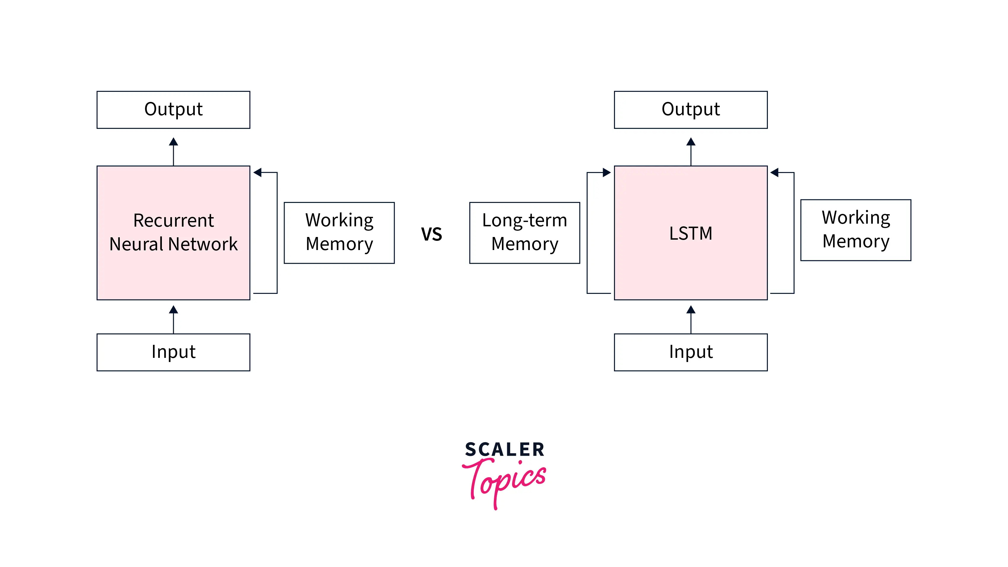
More specifically, along with maintaining the short-term memory of the context, LSTMs can also preserve the memory of context from time steps way behind in time and hence their name - long short-term memory networks.

Let us now look at the architectural details of the LSTMs and how they feature a gating mechanism that allows them to preserve long-term memory.

Working of the LSTM

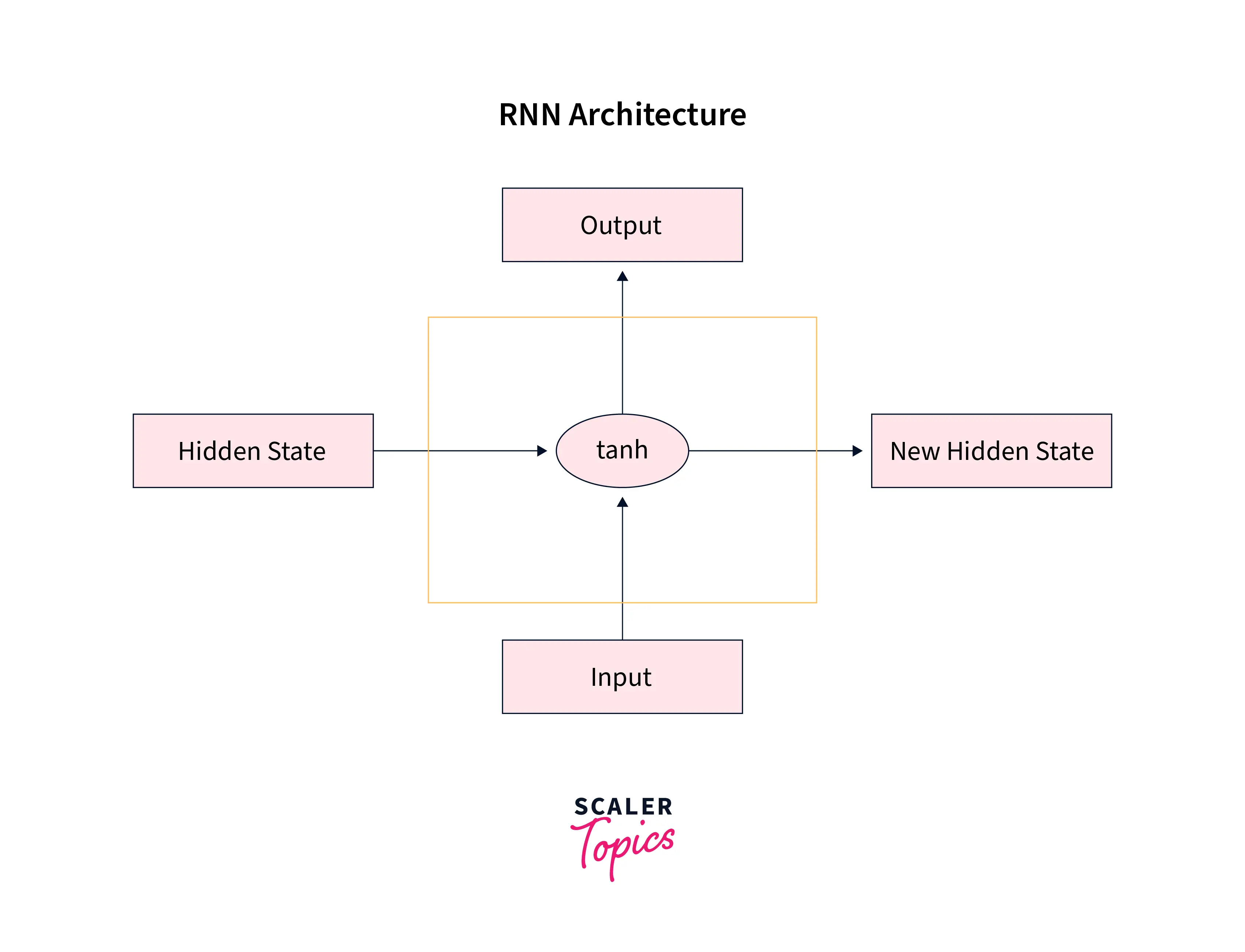
Suppose we recall the architecture of the vanilla RNN network. In that case, we know that the input at the current time step and the hidden state from the previous time step is passed through the tanh activation function to obtain the new hidden state for the current time step and also the output for the current time step.

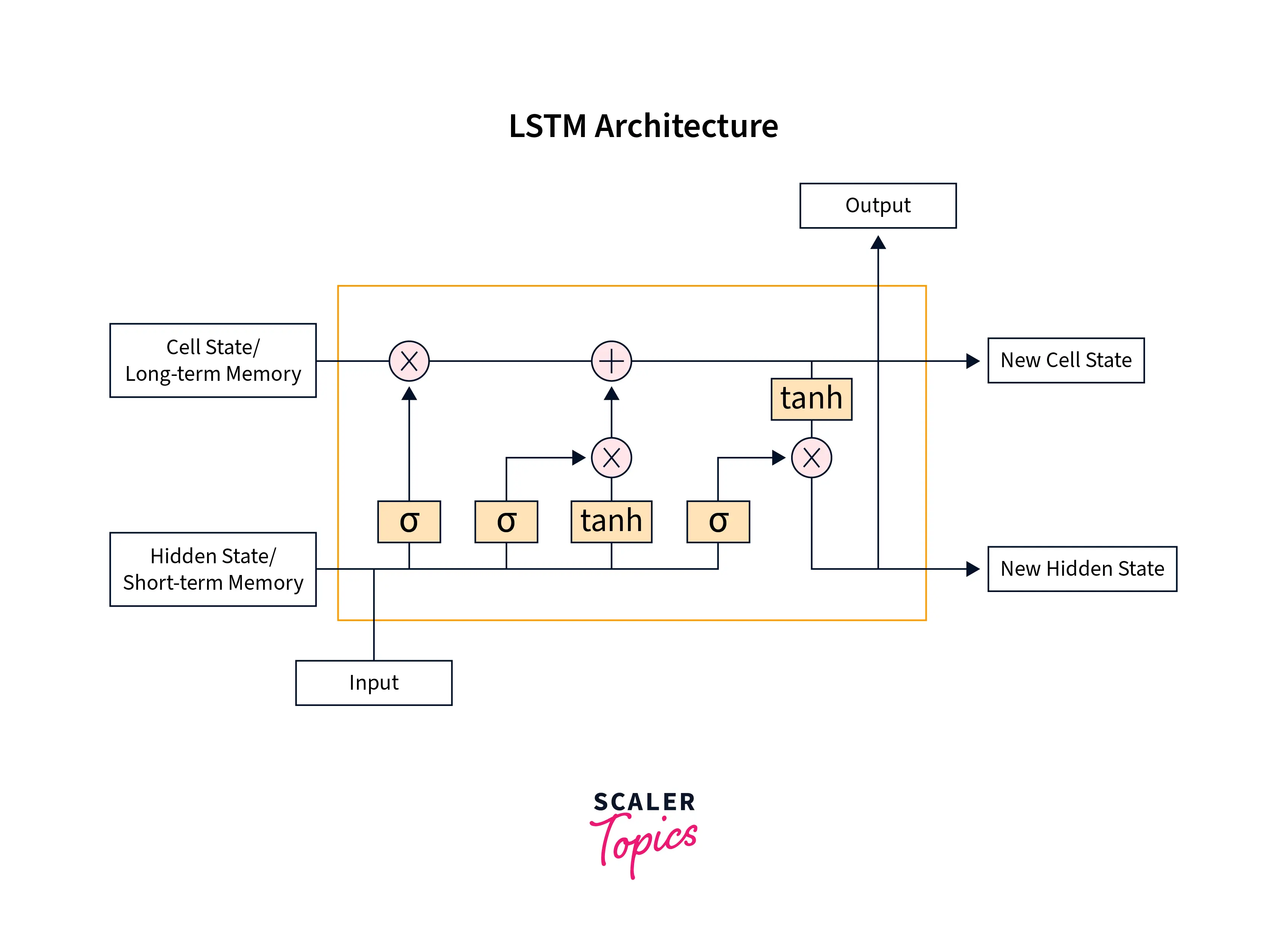
The architecture of LSTMs features one additional component called the cell state, which is used to maintain the memory from previous time steps far back in time. Specifically, at each time step, 3 components function together - the current input, the hidden state responsible for maintaining short-term memory, and the cell state responsible for maintaining short-term memory.

Special gates are included in the lstm cell to guard the flow of information from one time step to the other. These gates filter what information passes from one lstm cell to the other using the hidden and cell states.

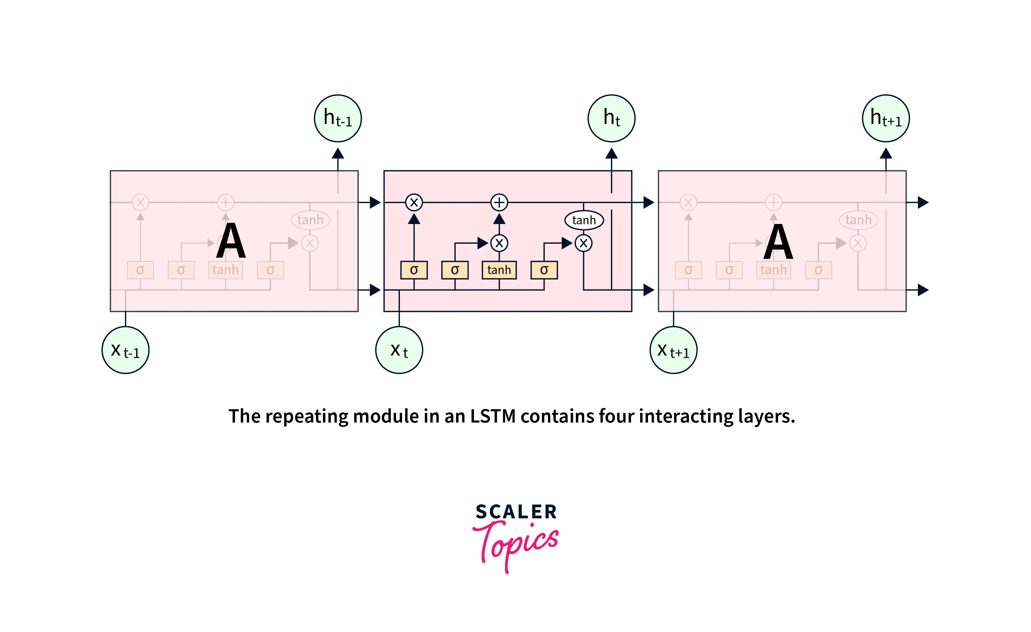
The three gates are the Input Gate, the Forget Gate, and the Output Gate. Architecturally, the flow of information through the lstm cell looks like the following -

Let us break down this architecture using the three gates we discussed above -

The Input Gate

The following sub-part of the network is called the input gate and is responsible for deciding what new information needs to be added to the long-term memory, which is being maintained by the cell state.

The input gate uses the current input and the short-term memory from the previous time step to filter out the information from these variables that is not useful in the long term. Then, it uses these two variables to update the cell state.

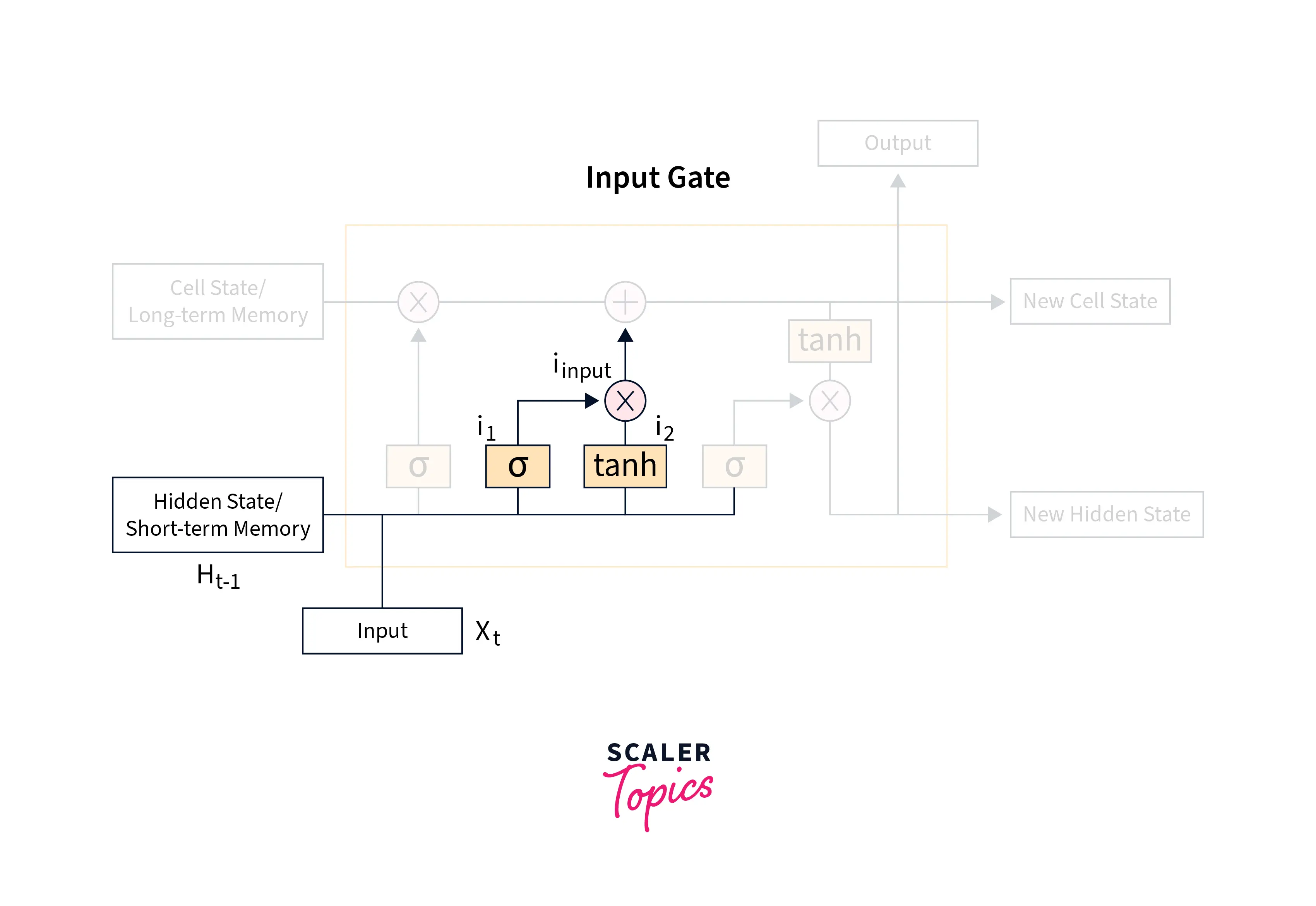
Mathematically, to control what information to retain and what to discard, the short-term memory and the current input are passed into a sigmoid function that maps the values to be between 0 and 1, where 0 indicates that that part of the information is unimportant and should be discarded, whereas 1 indicates that the information will be retained in maintaining the long term memory.

$i_1 = \sigma(W_{i_1} \cdot (H_{t-1}, x_t) + bias_{i_1})$

Another layer featuring the tanh activation function works with the current input and the short-term memory from the previous time step to regulate the network according to the following equation.

$i_2 = tanh(W_{i_2} \cdot (H_{t-1}, x_t) + bias_{i_2})$

Finally, these two are multiplied together to get the final output that will be used in the updation of long-term memory or the cell state, like so -

$i_{input} = i_1 * i_2$

The Forget gate

The forget gate is included in deciding what information from the long-term memory to keep or discard. It is done using a forget vector generated using the current input and incoming short-term memory and is used in multiplication with the incoming long-term memory.

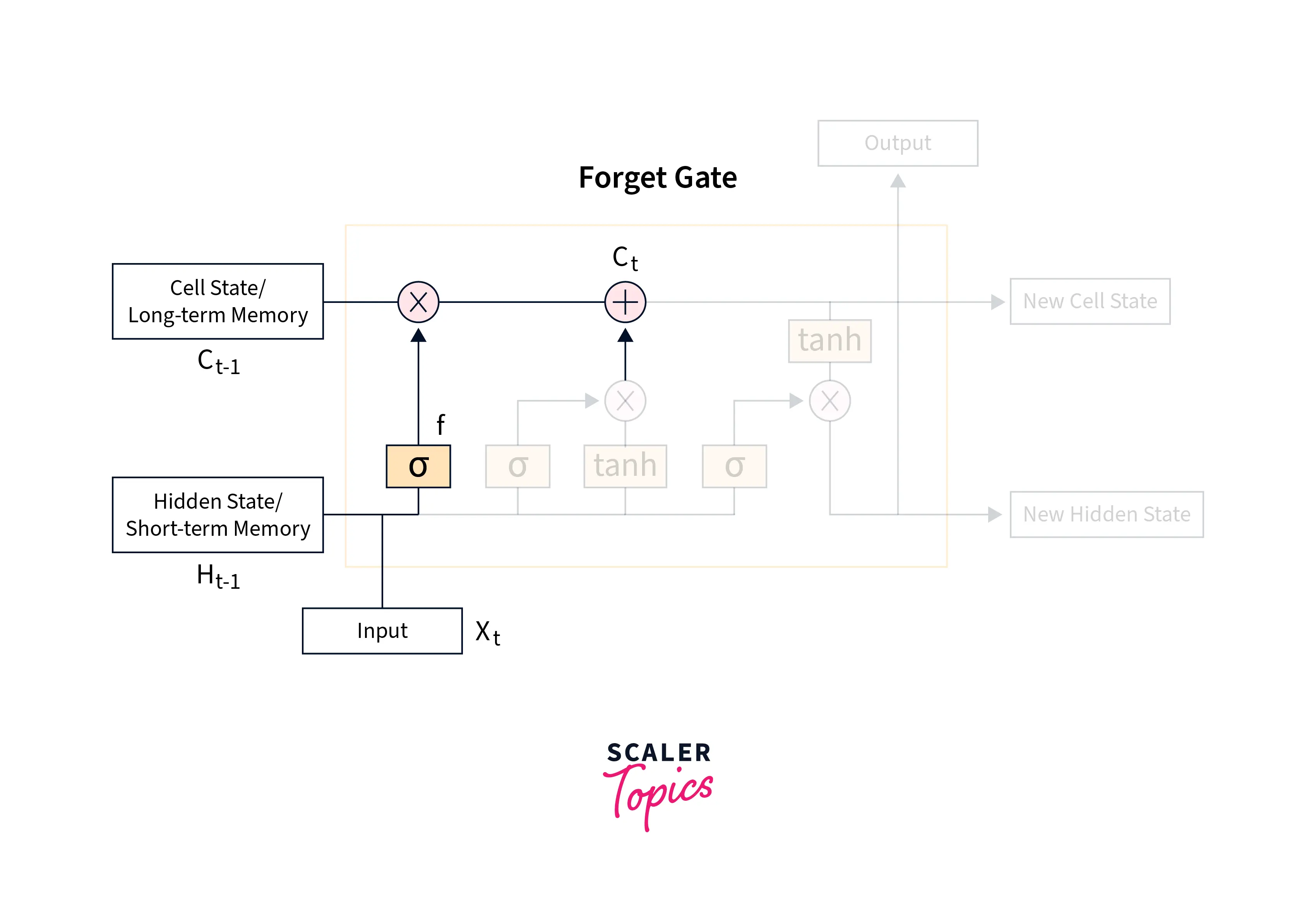
Mathematically, the forget vector is obtained by passing the short-term memory (or the hidden state vector from the previous time step) and the current input through a sigmoid function according to the following equation -

$f = \sigma(W_{forget} \cdot (H_{t-1}, x_t) + bias_{forget})$

Finally, the new cell state is obtained using the outputs from the Input gate and the Forget gate, like so -

$C_t = C_{t-1} * f + i_{input}$

Output gate

The Output gate is primarily meant to obtain the new short-term memory or the hidden state vector for the next time step by using the current input vector, the hidden vector from the last time step or the previous short-term memory, and the newly computed cell state or the long-term memory.

This gate is called so that it can also produce an output for the current time step.

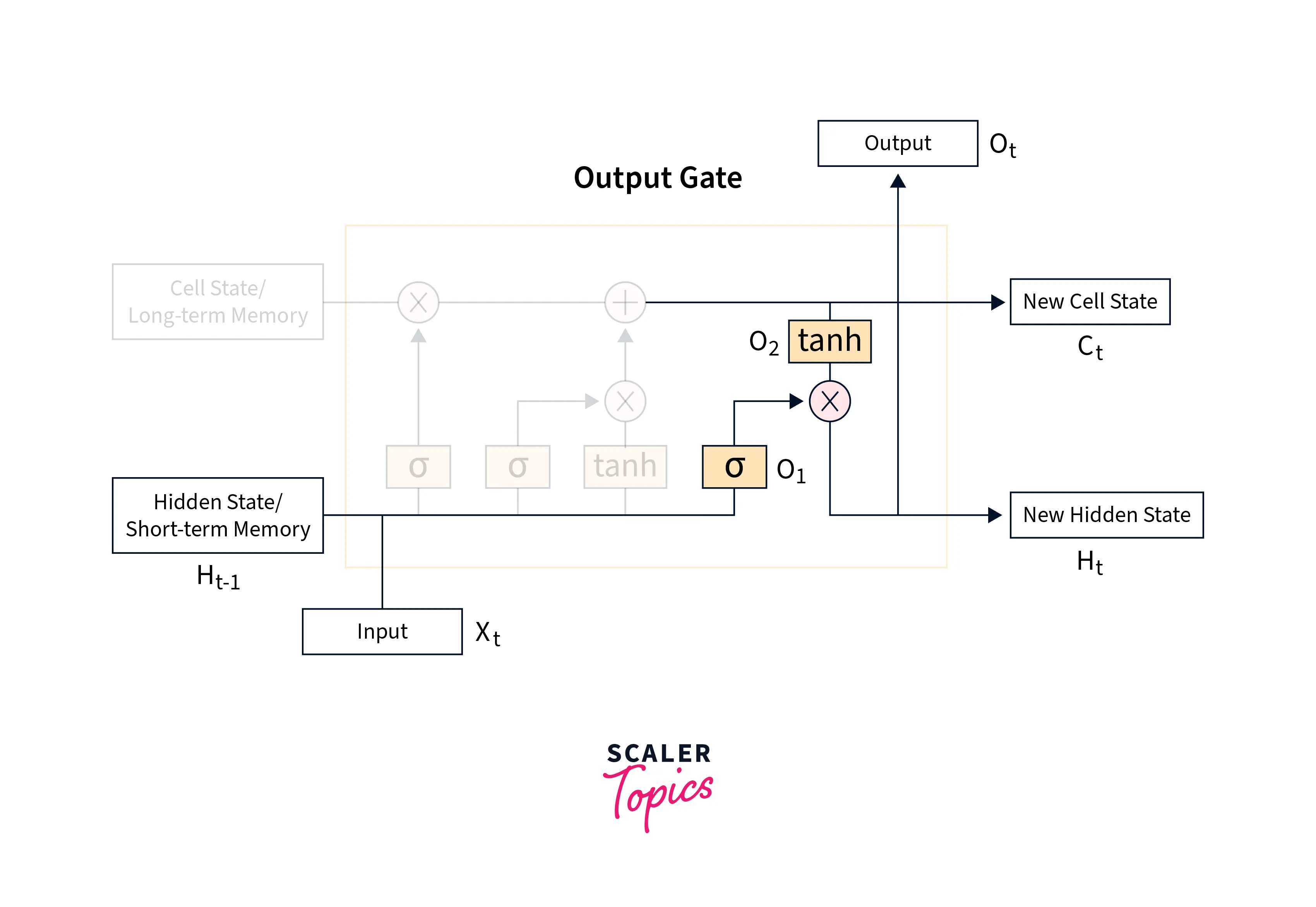
Mathematically, the previous hidden state and the current input will be passed into a sigmoid function as we've been doing the last two gates to create a filter, like so -

$O_1 = \sigma (W_{output_1} \cdot (H_{t-1}, x_t) + bias_{output_1})$

Then another layer uses the current cell state along with the tanh activation function to get another component, like so -

$O_2 = tanh(W_{output_2} \cdot C_t + bias_{output_2})$

Both of these components are now multiplied together to obtain the new hidden state, like so -

$H_t, O_t = O_1 * O_2$

The hidden state and the cell state produced are passed on to the next LSTM cell.

How to Use LSTM in PyTorch

We are now done understanding the architectural details of LSTM Networks. Let us now demonstrate the PyTorch API for LSTMs, after which we will implement a full-fledged LSTM PyTorch example.

The LSTM layer can be used via the torch.nn module, like so -

Here,

Input dimension - represents the size of the input at each time step,

Hidden dimension - represents the size of the hidden state and cell state at each time step

Number of layers - the number of LSTM layers stacked on top of each other

We will now create a dummy input vector to feed into our model and initialize a hidden and cell state. The hidden and cell states must be stored in a tuple like so - (hidden_state, cell_state).

We will now feed these into our lstm layer to get the output and hidden vector, like so -

Output:

Now that we have demonstrated the PyTorch LSTM API, we will now move on to implement an LSTM PyTorch example.

Generating the Data

We will be using the Reddit clean jokes dataset that is available for download here.

The dataset contains a collection of jokes in a CSV file format, and using the text sentences; our goal is to train an LSTM network to create a text generation model that will predict the next words given a series of words.

Importing Libraries

We will begin by importing all the necessary dependencies, like so -

The Dataset Class

after this, let us now define the custom dataset class to load individual samples of data from the file, like so -

The Model

we will now define a custom model class to define our lstm model. Our custom architecture also contains an embedding layer and a fully connected layer.

Training and Testing the Model

Let us now define a helper function to train our model containing the training loop like so -

We will also define a function to predict the next words and finally train our model and use the trained model for generating text like so -

Output:

Difference Between RNNs and LSTMS

Let us now go over the major points of differences between vanilla RNNs and LSTMs -

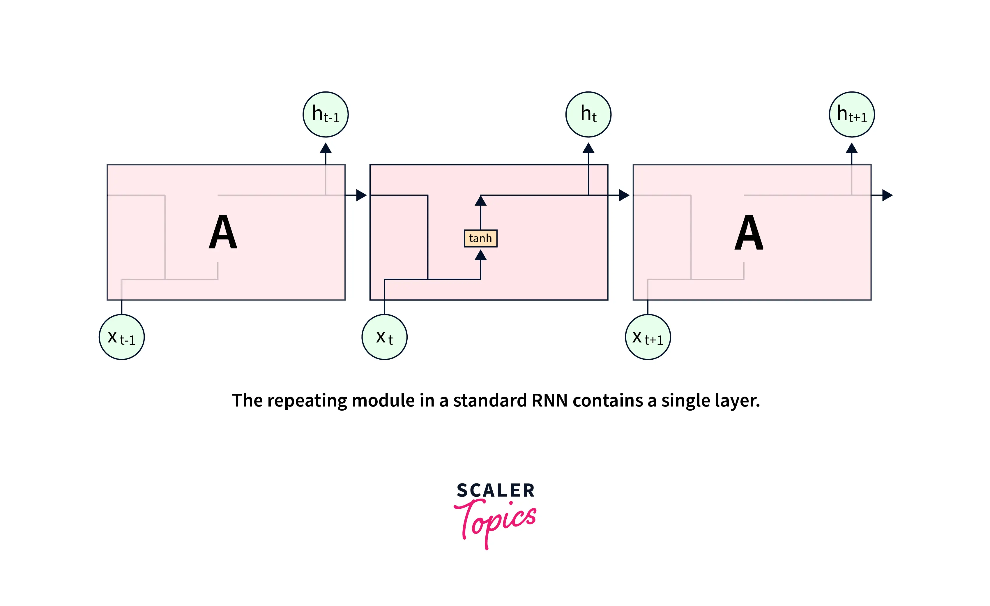
Architectural Differences

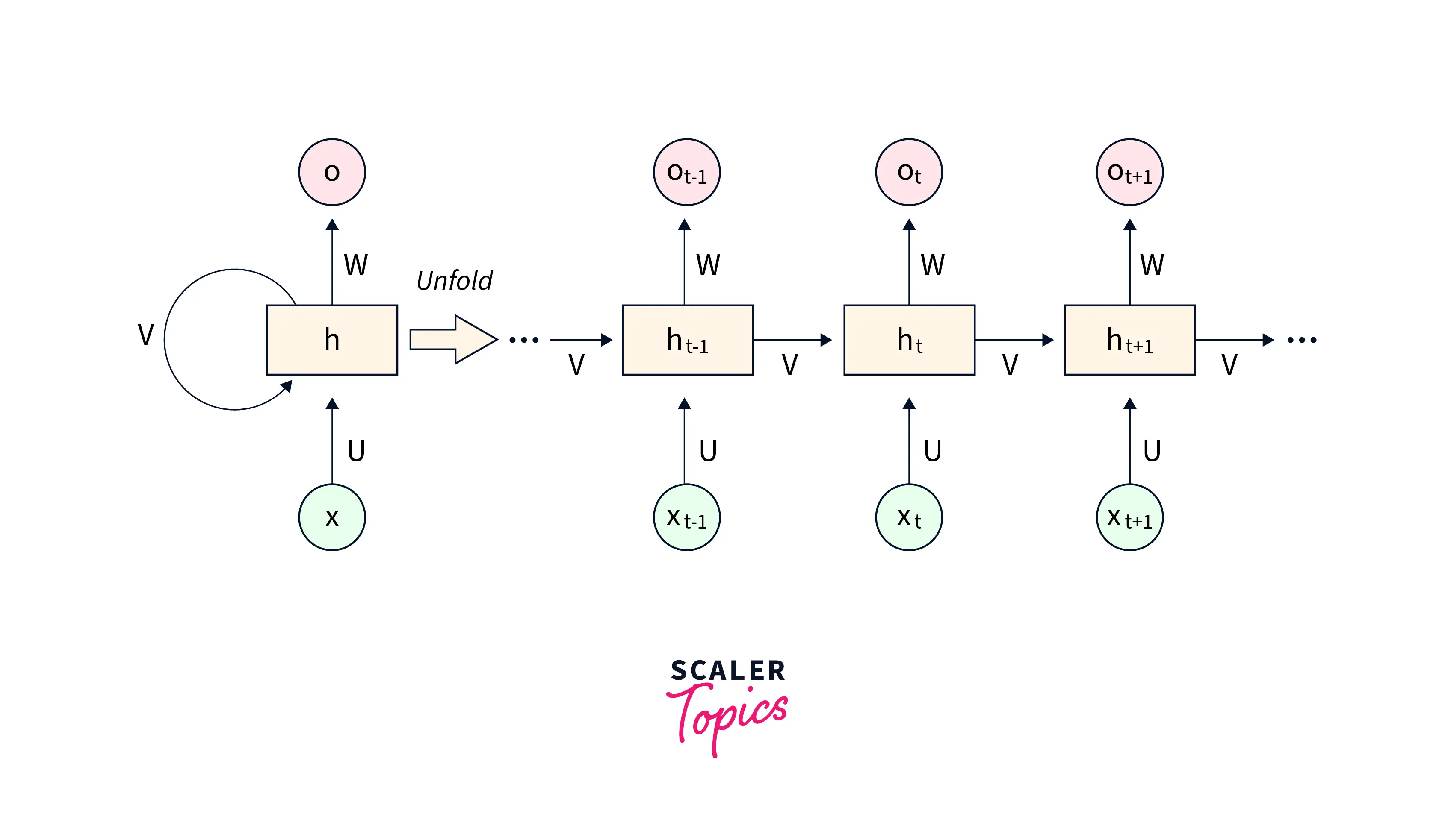
• Each unit of Vanilla RNNs features a simple activation function that updates the hidden state and produces the output at each time step. Following is the unrolled version of a vanilla RNN -

• LSTM units feature a 'memory cell' that is included to maintain information in the network's memory. The architecture also features a set of gates that control what information enters the memory, what information is output at a particular time step, and what amount of information is forgotten as we move further. Following is the unrolled version of an LSTM -

Owing to these architectural differences, there are two more major points of differences between vanilla RNNs and LSTMs as follows -

• Vanilla RNNs suffer from the vanishing gradient problem; hence, training them with longer sequences is challenging.
• LSTMs, on the other hand, due to their gated mechanism, do not suffer from the vanishing gradient problem to a great extent.
• RNNs, because of the vanishing gradient problem, cannot maintain the memory from long time steps back in time. They hence cannot capture the dependency between longer sequences leading to poor prediction performance.
• LSTMs are specially designed in a way such that they can capture the information from long back as the gates filter out selected information moving forward.

What is Bi-LSTM?

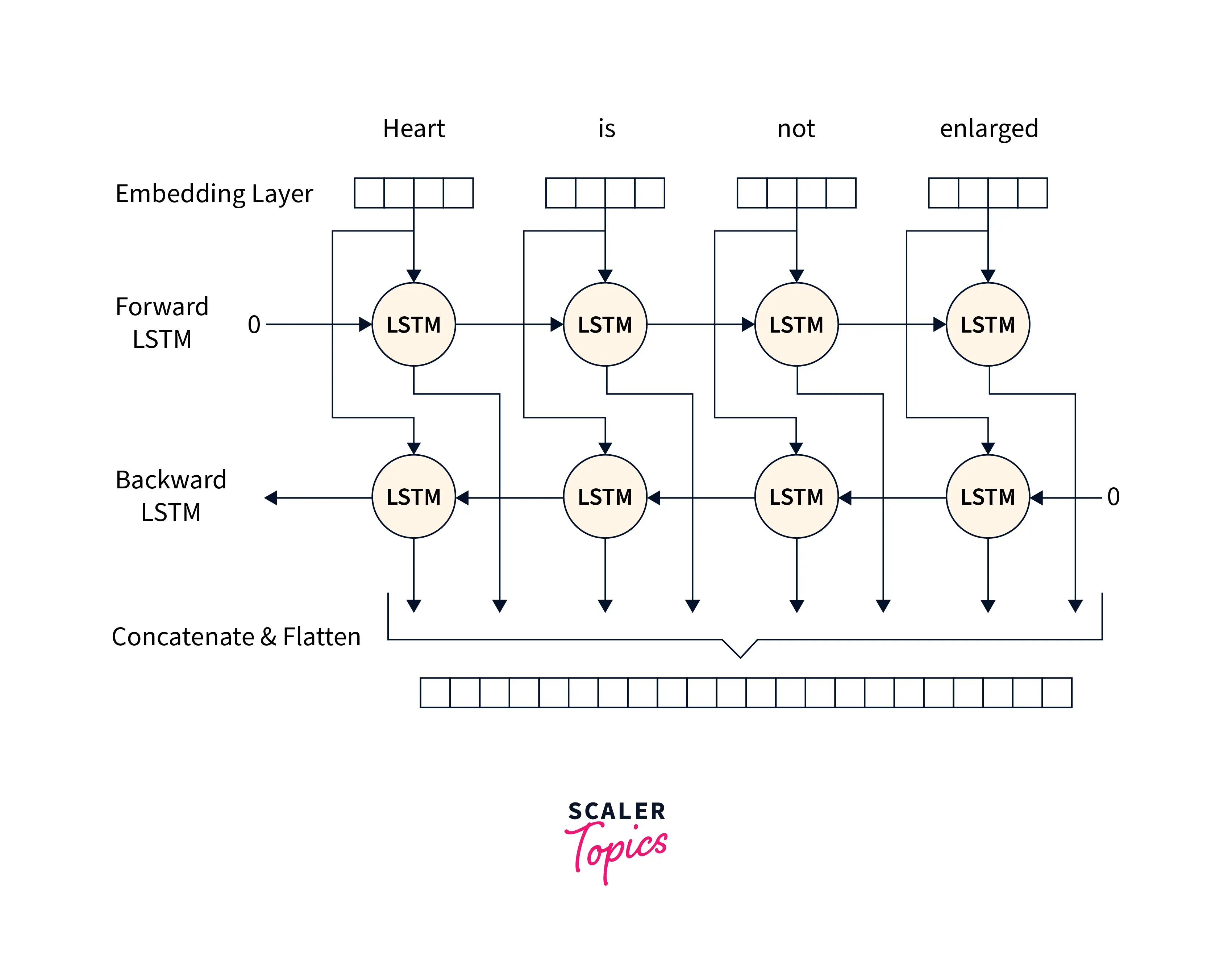
Bidirectional LSTMs are an extension of traditional LSTMs that can be used to improve model performance on tasks where all the sequence units shall be available, for example - sequence classification, speech recognition, and forecasting models. A Bidirectional LSTM, or biLSTM, is a model architecture used to process sequences, and it consists of two LSTMs: one of which takes the input in the forward direction, that is, it takes the input sentence as it is, and the other one takes the reverse sequence as input, in the backward direction.

This way, Bi-LSTMs leverage more information to train the network with an increased context available for the model to learn from.

As we know, context matters when modeling sequential data. However, it is the context from both ends that matter. For example, to build a model to fill in empty blanks of text sequences, for example - the boys are ______ cricket, all four words form contextual information for the model to use while predicting what word shall fit in the blank.

While LSTMs can process the context only from one direction, BiLSTMs employ two LSTMs in a single architecture to use context from both sides of a sequence.

Implementing the Bi-LSTM Architecture with PyTorch

Let us now Implement the Bi-LSTM Architecture with PyTorch. We will first set the correct hardware device along with importing all the dependencies, like so -

After this, we will set some hyperparameters and variables required to build and train our model -

Let us now load the dataset splits and create dataloader instances for them. for this example, we are using the good old MNIST dataset, which is easily available for downloading using the torchvision module.

We will now define our custom model class by inheriting the base class nn.Module, like so -

To prepare for training of our network, we will now create the model instance and define the optimization algorithm along with the criterion for updating the model parameters like so -

Let us now define a training loop for our model to train the bi lstm model we defined -

With this, our model is trained, and we are now left to check the model's performance on unseen test data. We will define a simple function to do that, like so -

Output:

That was all about using a Bidirectional LSTM using the PyTorch API.

Review the major differences between a plain LSTM architecture and a Bidirectional LSTM.

LSTM vs. Bi-LSTM

The major point of difference between LSTM vs. Bi-LSTM is in their architectures that allow Bi-LSTMs to use context from both ends in a sequence.

Specifically, unidirectional LSTMs can preserve information from input units that have already passed through it using the hidden state, that is, from the previous time steps.

With bidirectional LSTMs, we run the input sequence through the network in two ways once the sequence is processed as it is. Once the reversed sequence is processed by which, we get two hidden states combining which we can preserve information from both past and future.

Elevate your deep learning skills with PyTorch. Join our Free PyTorch for Deep Learning Course now and stay ahead in AI.