Quick Sort in C++

Introduction
As the name suggests, a quick sort algorithm is known to sort an array of elements much faster (twice or thrice times) than various sorting algorithms.
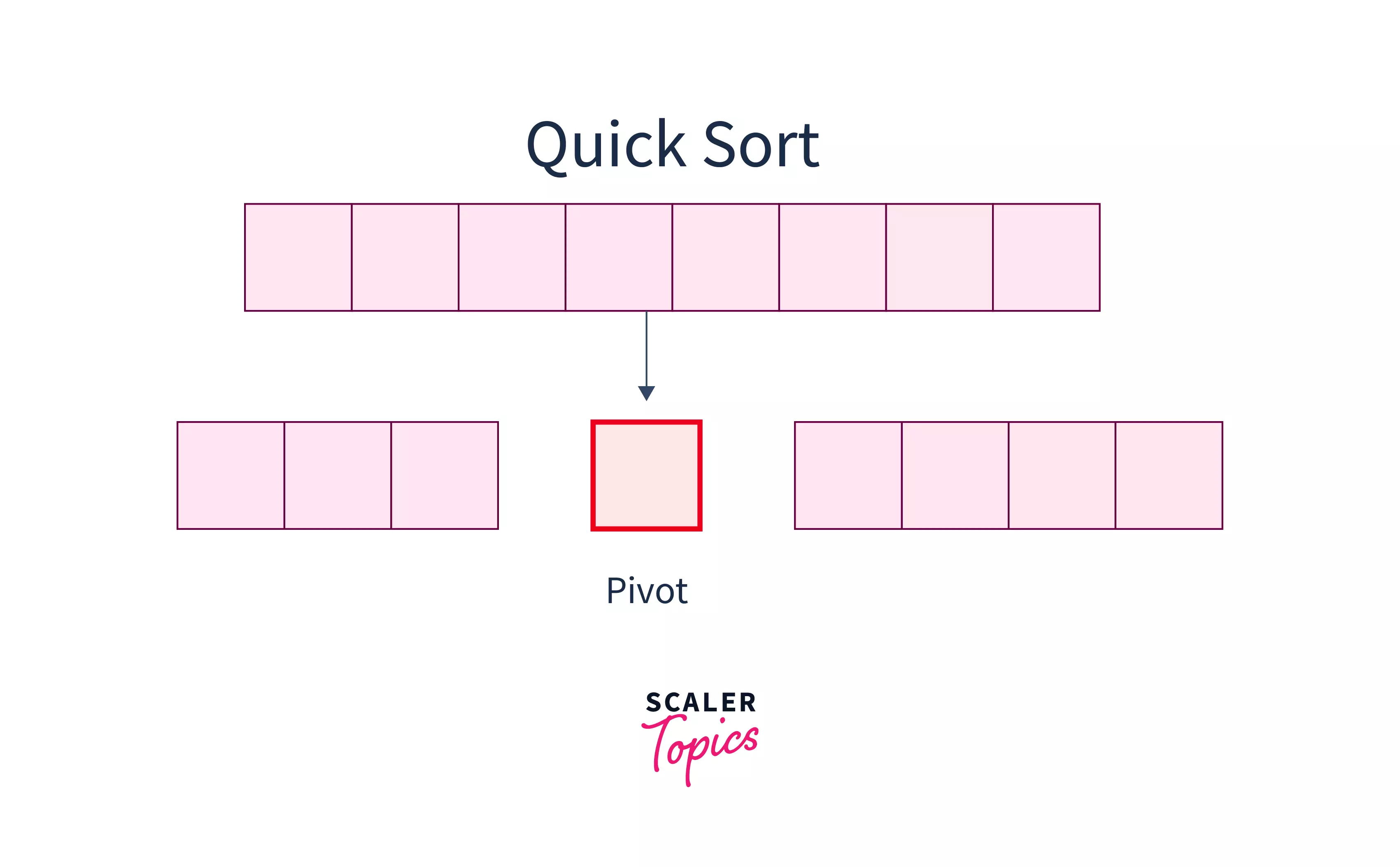
Quick sort uses the divide and conquer technique where we partition the array around an element known as the pivot element, which is chosen randomly from the array. We solve the partitions to achieve an ordered array. Due to this reason, it is also known as the Partition Exchange Algorithm. A similar algorithmn to Quick Sort is Merge Sort.
Working of Quick Sort Algorithm In C++
The quick sort algorithm works in a divide-and-conquer fashion :
- Divide :-
Choose a pivot element first from the array. After that, divide the array into two subarrays, with each element in the left sub-array being less than or equal to the pivot element and each element in the right sub-array being greater. This will continue until only a single element is left in the sub-array.
- Conquer :
Recursively, sort the two subarrays formed with a quick sort.
- Merge :
Merge the already sorted array.
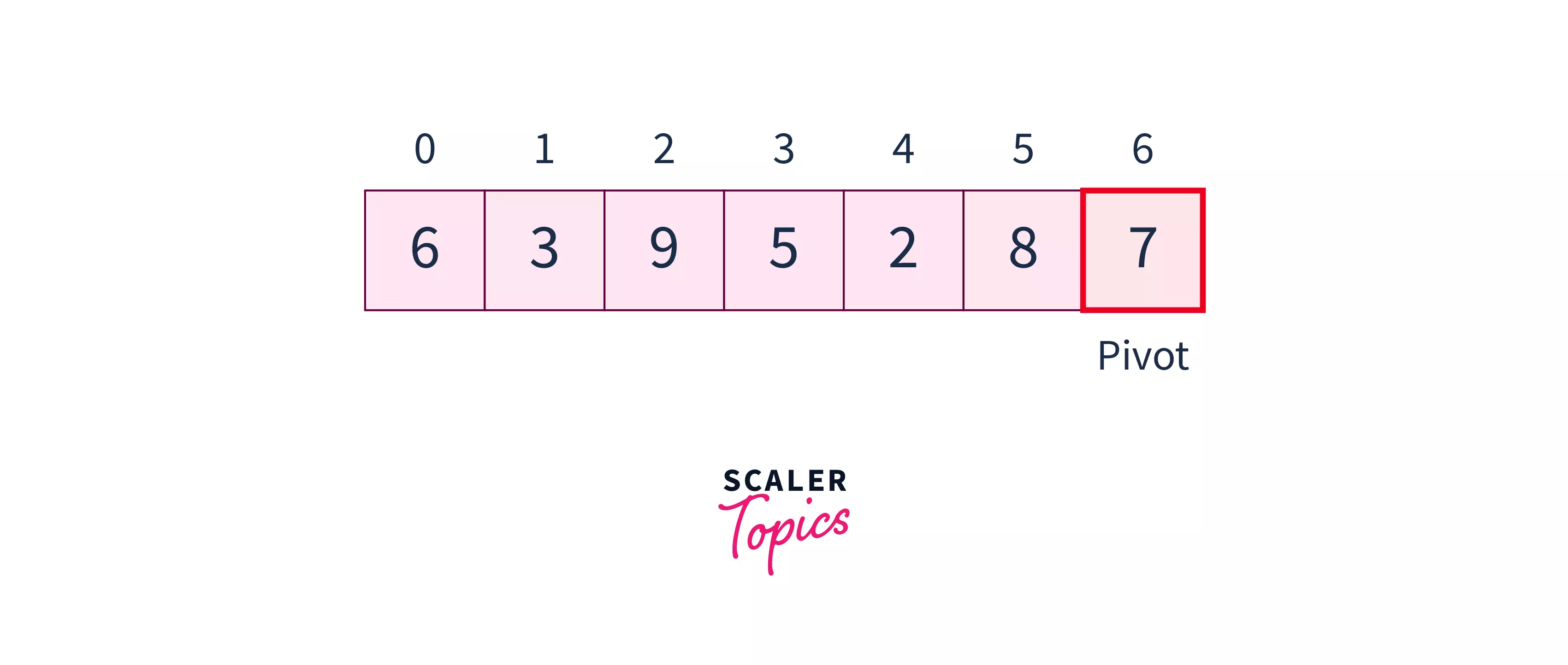
To discuss the working of the quick sort algorithm, let us take an example of an array:
- Select the pivot element:-
Firstly, we choose a pivot element from the element. There are many different ways of choosing a pivot element : * Pick the first element as pivot always. * Pick the last element as pivot always. * Pick a random element as a pivot. * Pick median element as pivot.
In this article, we will consider the last element of the array as the pivot element.
- Rearrange the array:-
We will rearrange the array such that elements smaller than the pivot element will come before the pivot element, and elements larger than the pivot element will come after the pivot element. Hence pivot element will come to its actual position.
In the above example, elements will come after , and will come before .
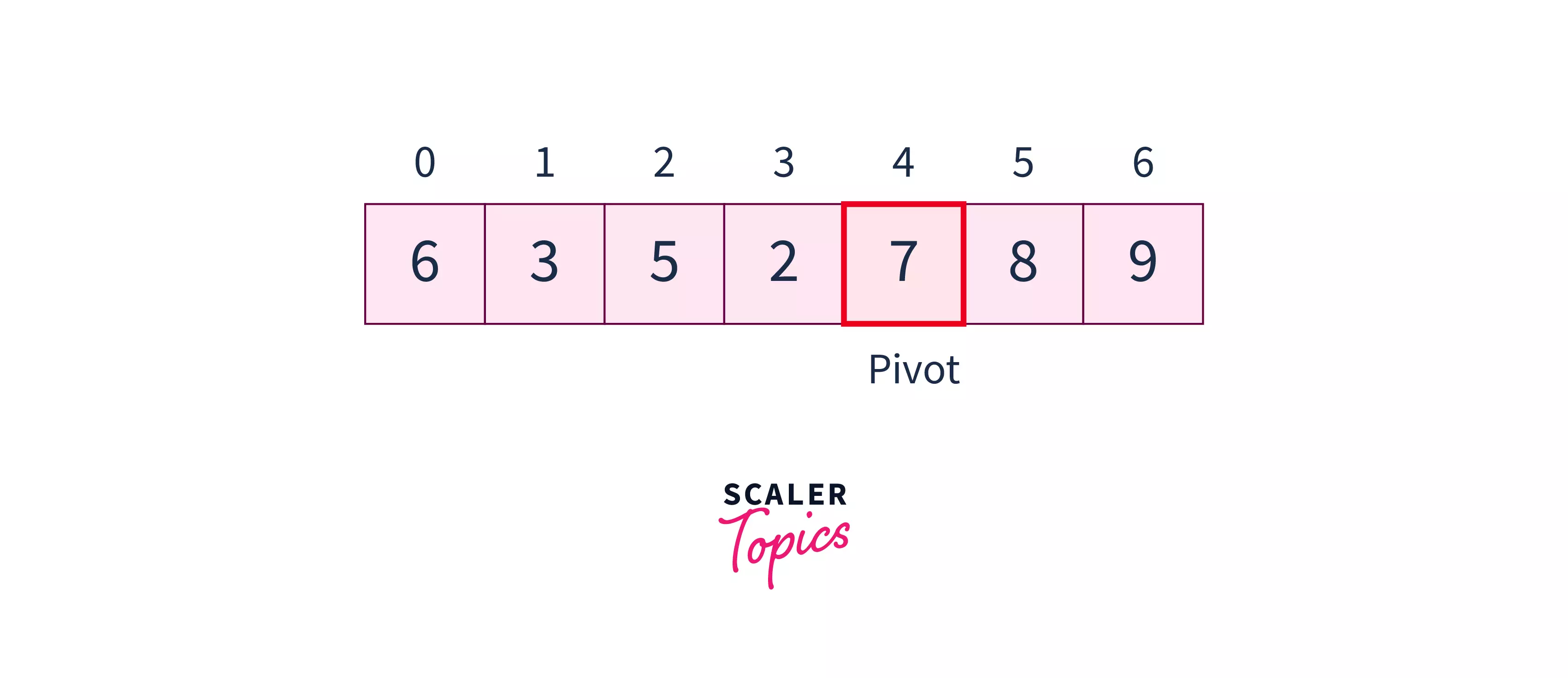
We rearrange the array in the following way :
- We initialize a pointer PIndex at index 0. This pointer will finally point to the pivot element's actual position.
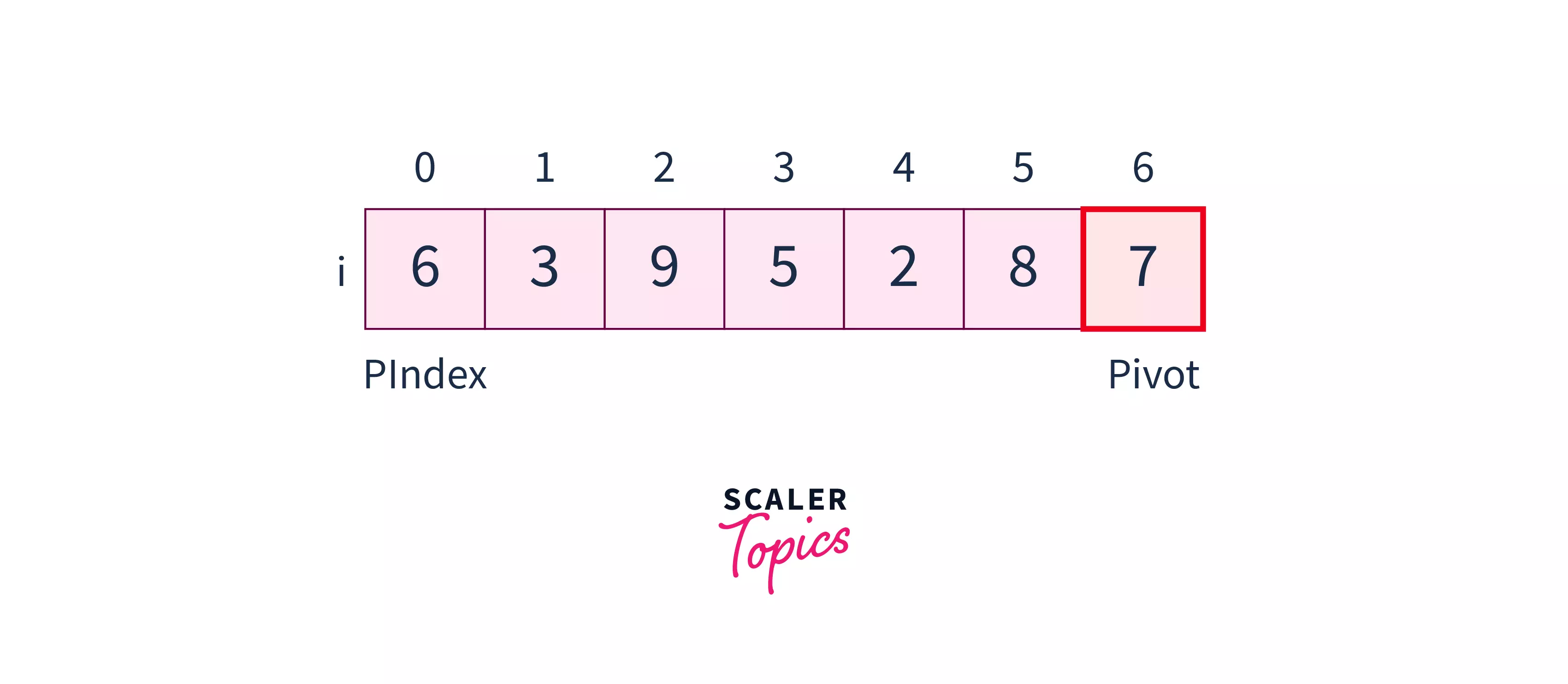
- Then we traverse the array till Pivot with a pointer. Let us say i and check for the following condition :
This way, we put all the smaller elements to the left of PIndex and all the larger elements to the right of the PIndex.
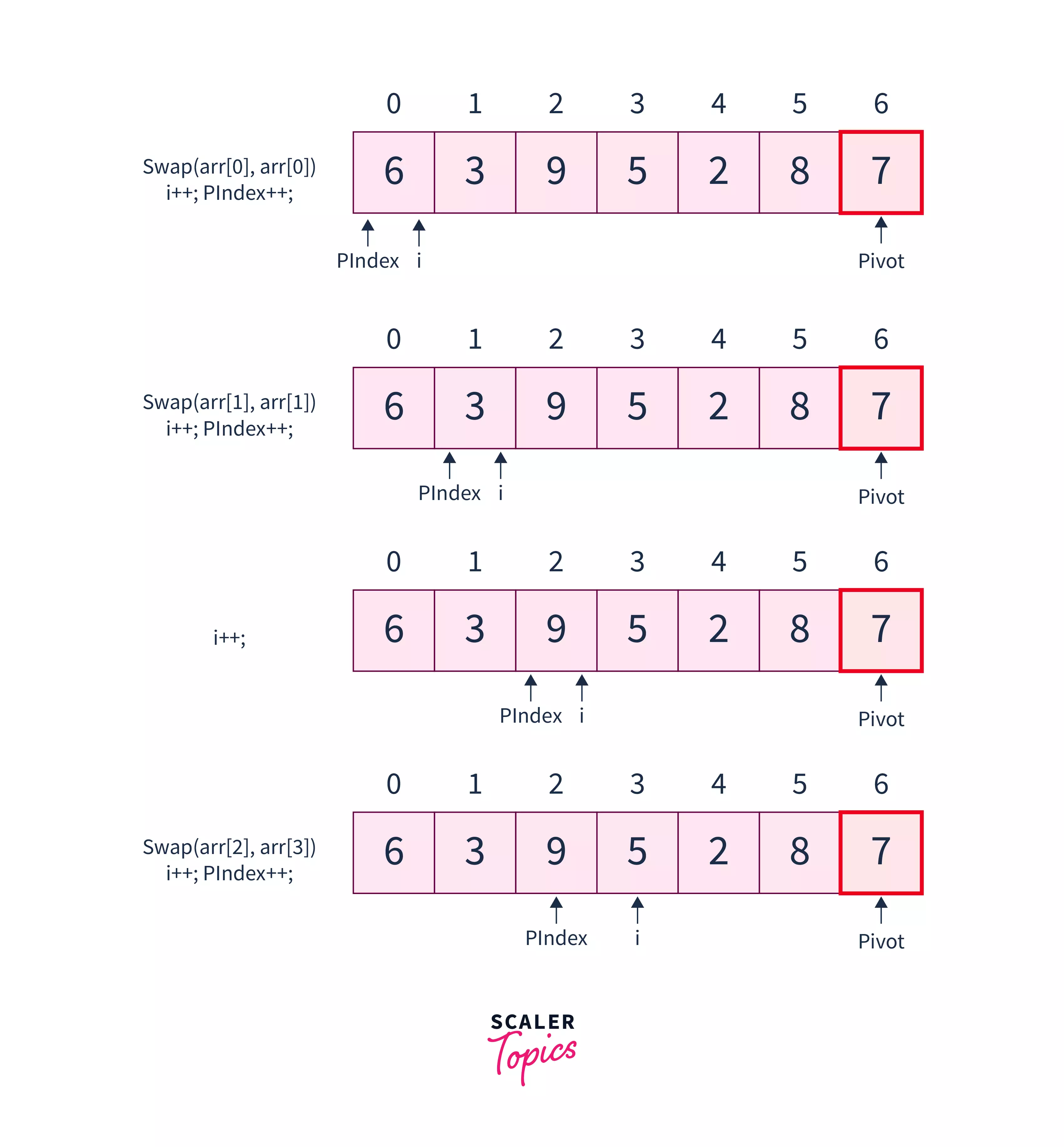
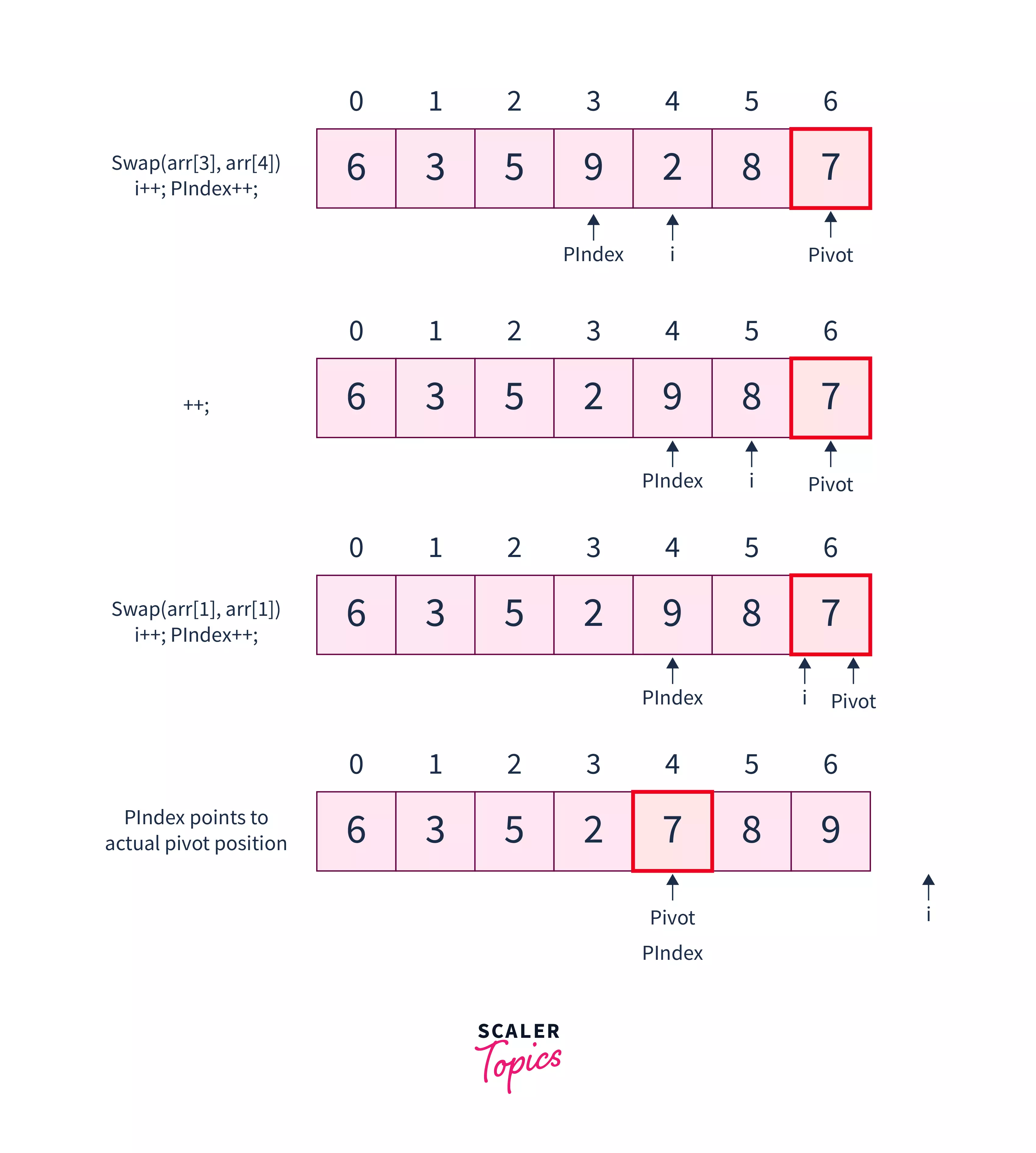
- After array traversal and swapping, do PIndex= PIndex-1. This way, we rearranged the elements by partitioning the array into two subarrays- one to the left of the PIndex and one to the right of the PIndex.
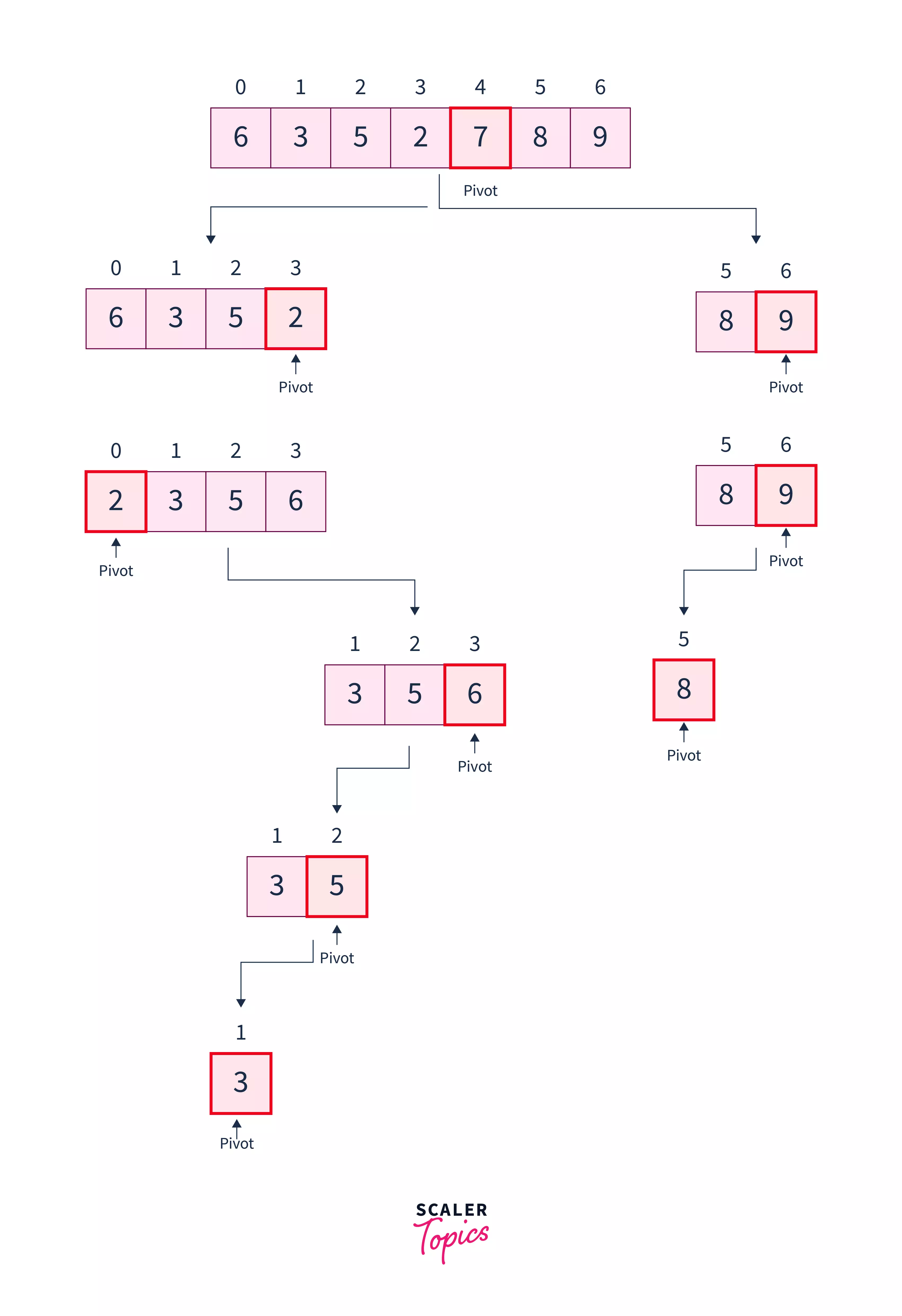
- Divide Subarrays: We pass the pivot index's left and right subarray recursively to the same process followed above. Therefore, in the above example, we pass subarray - [0 to 3] with pivot element as and subarray - [5 to 6] with pivot element as as the argument to the quickSort function again.
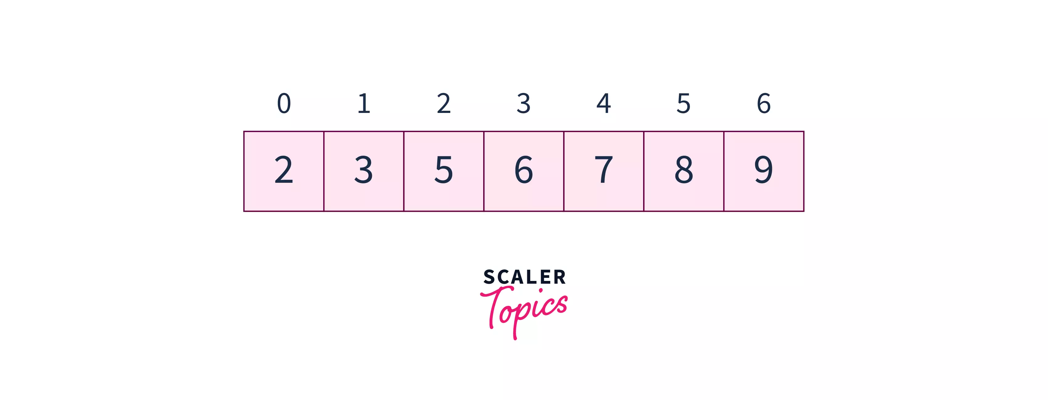
Sorted Array:
Transform Your Career
Choose from our industry-leading programs designed for career success
Modern Software and AI Engineering Program
Master full-stack development with AI integration

Modern Data Science and ML with specialisation in AI
Advanced data science techniques with AI specialization
Advanced AIML with Specialisation in Agentic AI
Deep dive into AIML with focus on Agentic systems
DevOps, Cloud & AI Platform Engineering
Build and manage AI-powered cloud infrastructure
AI Engineering Advanced Certification by IIT-Roorkee
Premier AI engineering certification from IIT-Roorkee
Implementation Of Quicksort In C++
- Firstly, we initiate two pointers, lo and hi, to the leftmost and rightmost elements of the array.
- Then, we call the partition function, which rearranges the array such that all the smaller elements are left to the pivot element and all the larger elements are right to the pivot element.
It returns the final pivot index PIndex in the range [lo, hi].
- Recursively call the quicksort for the left subarray of Pindex and the right subarray of the Pindex.
Pseudo Code :
C++ Code :
Output :
Scaler Placement Report and Statistics
Scaler learners achieved 2.5x salary growth with average post-Scaler CTC reaching ₹23L.
Quick Sort Complexity
- Time Complexity
| Case | Complexity |
|---|---|
| Best Case | |
| Average Case | |
| Worst Case |
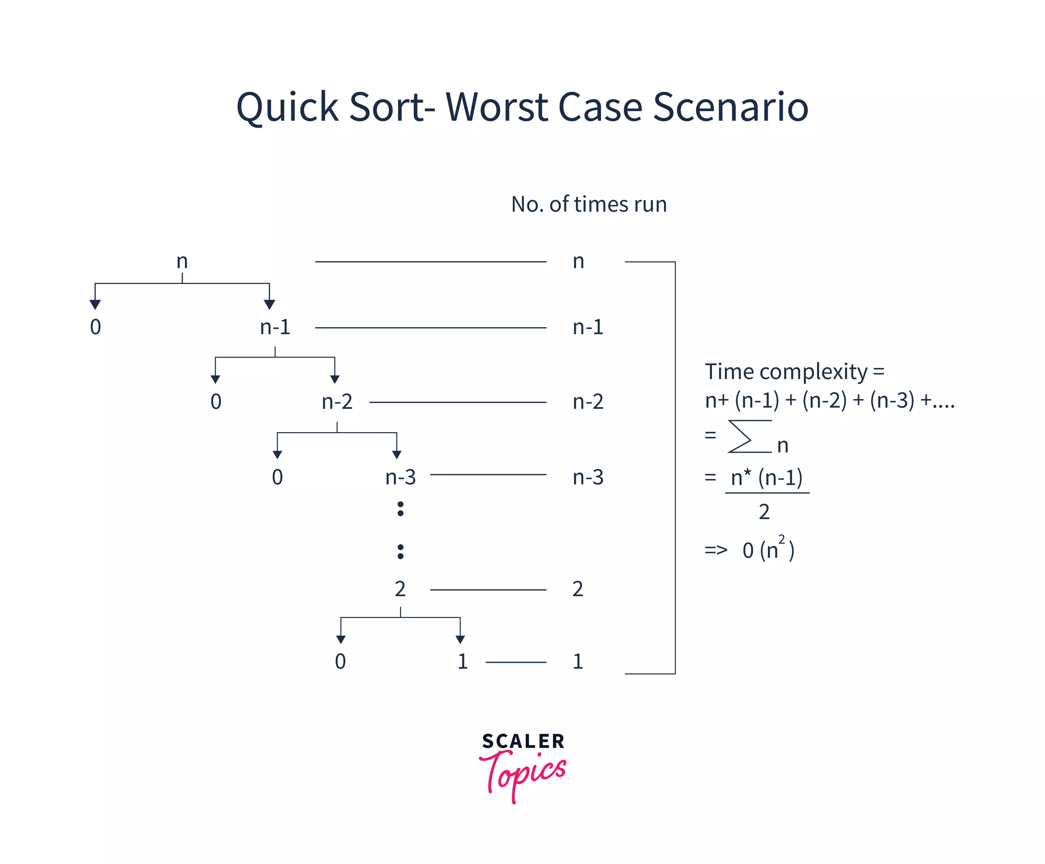
- Worst-Case Complexity:
In quick sort, worst-case complexity arises when the array is already sorted and the chosen pivot element is either the array's last or first element.
For example, if the array is and the pivot is chosen as the leftmost element, we always get the pivot index as the first element. If the pivot index is the first element of the sorted array, recursion stack branches in the ratio give rise to levels of the recursion tree.
Hence, Quicksort's worst-case time complexity is .
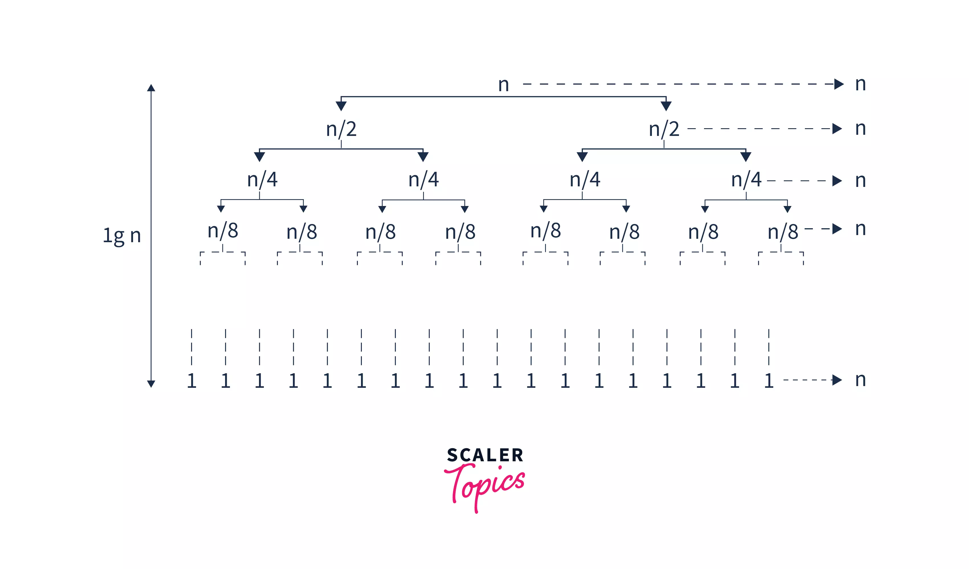
- Best-case complexity:
Arises when the pivot element is the middle element or close to the middle element in a quick sort. When the pivot index is found in the middle, the recursion branch spreads more evenly; hence, levels of the recursion tree are achieved.
Therefore, the best case time complexity is .
- Average Case Complexity :
It occurs when the array elements are not sorted at all. In other words, the array is fully unordered.
In this case, the average case scenario is similar to the best-case scenario as the jumbled array also gives an evenly divided recursion stack. Hence, Quicksort's average case time complexity is .
- Space Complexity
| Case | Complexity |
|---|---|
| Best Case | |
| Average Case | |
| Worst Case |
As the algorithm is in place, where we sort the array in the original array, space complexity arises only because of the recursion stack. So, there must be a call stack entry for every one of these function calls.
This means that with an array of n integers, at worst, there will be n stack entries created, hence worst-case space complexity.
The average case space complexity arises when we create call stack entries. Hence average space complexity is .
Characteristics Of Quick Sort
- A stable sorting algorithm :
Maintains the position of two equal elements relative to one another. Quick sort is not a stable algorithm because elements are swapped according to the pivot’s position (without considering their original positions).
- Quick sort algorithm is an in-place algorithm, which means array elements are sorted in the original array. In other words, the array is modified in the original array itself.
- Quick sort is an algorithm for quickly and efficiently sorting an array or list. Because the algorithm is always in place, quick sort is used when the space is limited.
Turn Learning into Career Growth
3-Way Quick sort (Dutch National flag)
In simple quick sort, we partition the array around the pivot element and recurse for the left and the right subarrays.
So, when array contains redundant elements with multiple occurrences like with chosen pivot as 1 then we will be setting only one occurrence of 1 to its actual position in one recursive call.
To avoid this complexity, we use the 3-way Quick Sort algorithm, which partitions the array arr[l..r] into 3 subarrays :
- arr[l...i] : Left subarray with elements less than the pivot element.
- arr[i+1...j-1] : Subarray with elements equal to the pivot element.
- arr[j...r] : Right subarray with elements greater than the pivot element.
Through this, we set the actual position of all the occurrences of 1 in a single pass. Thus 3-way quick sort can be used when we have more than one redundant element in the array.
Pseudo Code :
- partition(arr, left, right, i, j) :
- quicksort(arr, left, right) :
Randomized Quick Sort
Sometimes it happens when choosing the rightmost element in the sorted array as a pivot, resulting in a worst-case time complexity of .
In such cases, we use randomized quick sort algorithm, which is nothing but choosing a random pivot element from the array. Here we are probably choosing a pivot near the center of the array, and when this happens, the recursion branches spread more evenly, making it fast to sort the array elements in time.
Pseudocode(Lomuto partitioning) :
Note :
- Using random pivoting, we improve the expected or average time complexity to . The Worst-Case complexity is still .
- In internal sorting, all the data to sort is stored in memory at all times while sorting is in progress. In external sorting, data is stored outside memory (like on secondary memory) and only loaded into memory in small chunks.
Quick Sort vs. Merge Sort
| Features | Quick sort | Merge sort |
|---|---|---|
| Partitions | The array is split into two parts around a pivot element and can be partitioned into any ratio. | The array is partitioned into two halves. |
| Worst case complexity | - We need to make many comparisons in the worst-case scenario. | – same as the average case scenario. |
| Data sets usage | It is not efficient for larger data sets. | It is efficient for all the data sets irrespective of size. |
| Additional space | Inplace – no need for additional space. | Not in place – needs additional space to store auxiliary array. |
| Sorting method | Internal – data is sorted in the main memory. | External – external memory is used for storing data arrays. |
| Efficiency | Faster and efficient for small size array. | Fast and efficient for larger array and smaller both. |
| Stability | Not stable as two elements with the same values will not be placed relatively in the same order. | Stable as two elements with the same values will appear in the same order in the sorted array. |
| Arrays/linked lists | More preferred for arrays. | Works well for linked lists. |
Conclusion
-
Quick sort in c++ uses the divide and conquer technique to sort elements of the array much faster than other sorting algorithms. It is also known as the Partition Exchange Algorithm.
-
We sort them by choosing a pivot, rearranging the array around it, and then calling recursively for both left and right subarrays around the pivot.
-
Quicksort's best-case time complexity is . In the worst-case scenario, it becomes when all the elements are already sorted. The worst-case space complexity is for quicksort.
-
It is an in-place algorithm where sorting is done in the original array (cache-friendly).
-
We use the 3-way quick sort technique for redundant array elements.
-
We improve the worst-case scenario of a simple, quick sort by choosing a random pivot from the array(randomized quicksort).
-
Quick sort in C++ does not always partition the array into two halves, whereas, in merge sort, the partition is always into two halves.
-
In the real world, quicksort is generally used in commercial computing, numerical computations, and information search.
-
It is an unstable algorithm that does not preserve the relative ordering of the same elements from the original array.