Shortest Job First (SJF) in Operating System
Overview
An Operating System uses a variety of algorithms to efficiently arrange the operations for the processor, Shortest Job First (SJF) algorithm is one of them. In the Shortest Job First algorithm, the CPU will be assigned a job with the smallest burst time first, and the processes in the queue with the shorter burst time will be received and executed by the CPU more quickly. We'll discuss an in-depth explanation of the SJF scheduling algorithm with examples in the below article.
What is the Shortest Job First Scheduling in the Operating System?
Shortest Job First (SJF) algorithm is also known as Shortest Job Next (SJN) or Shortest Process Next (SPN). It is a CPU processes scheduling algorithm that sorts and executes the process with the smallest execution time first and then the subsequent processes with the increased execution time. Both preemptive and non-preemptive scheduling strategies are possible in the SJF scheduling algorithm. In SJF, there is a significant amount of reduction in the average waiting time for other processes that are waiting to be executed.
However, it can be quite challenging to estimate the burst time required for a process, making it difficult to apply this technique to the operating system scheduling process.
The burst time for a process can only be approximated or predicted. To get the most out of the SJF algorithm, our approximations must be correct. Numerous methods can be used to predict a process's CPU burst time.
1. Static Techniques:
- Process Size: We approximate the burst time of the upcoming process by using the burst time of an older process having a similar size.
- Process Type: Depending on the type of the process, we can estimate the burst time. There are several different sorts of processes, , for example,, Background Processes, User Processes, Operating System Processes, etc.
2. Dynamic Techniques:
- Simple Averaging: In simple averaging, a list of processes is provided. , ,.......,. Let represent the process's burst time. Let be the estimated burst time for the process. The estimated burst time of a process can be determined by:
where, and is the summation of all the burst times and .
- Exponential Averaging or Aging: Let represents the process's exact burst time. If the process's estimated burst time is , the subsequent process's CPU burst time can be determined by:
where represents the smoothing. Its value ranges from to .
Characteristics of SJF Scheduling
The following are the characteristics of Shortest Job First Scheduling:
- Shortest Job First has the shortest average waiting time out of all scheduling methods.
- SJF is categorized as a Greedy algorithm.
- The Starvation problem can occur if shorter processes continue to be generated, to solve this we can use an ageing technique.
- The operating system can't calculate the burst times, so it is almost impossible to sort them. Although execution time cannot be calculated, it can be estimated using a variety of techniques, such as a weighted average of earlier execution times.
- This algorithm can be utilized in specialized environments where precise burst time (or running time of an application) estimations are available.
Transform Your Career
Choose from our industry-leading programs designed for career success
Modern Software and AI Engineering Program
Master full-stack development with AI integration

Modern Data Science and ML with specialisation in AI
Advanced data science techniques with AI specialization
Advanced AIML with Specialisation in Agentic AI
Deep dive into AIML with focus on Agentic systems
DevOps, Cloud & AI Platform Engineering
Build and manage AI-powered cloud infrastructure
AI Engineering Advanced Certification by IIT-Roorkee
Premier AI engineering certification from IIT-Roorkee
SJF Algorithm
The Algorithm for Shortest Job First CPU Scheduling is as follows:
- First sort all the CPU processes in order of their arrival time to identify the one that needs to be executed first. This makes sure that the process that came first and had the shortest burst duration is the one that is executed.
- Segment Trees are used to find the minimum burst time process from all the arriving processes rather than iterating over the entire struct array to identify the minimum burst time process among all the arrived processes.
- After choosing a process that needs to be executed, the arrival time and burst time of the process are used to compute the different times, for example, the turnaround time of a process, the waiting time of a process, and the completion time (all the times are discussed in the next section of this article).
Example:
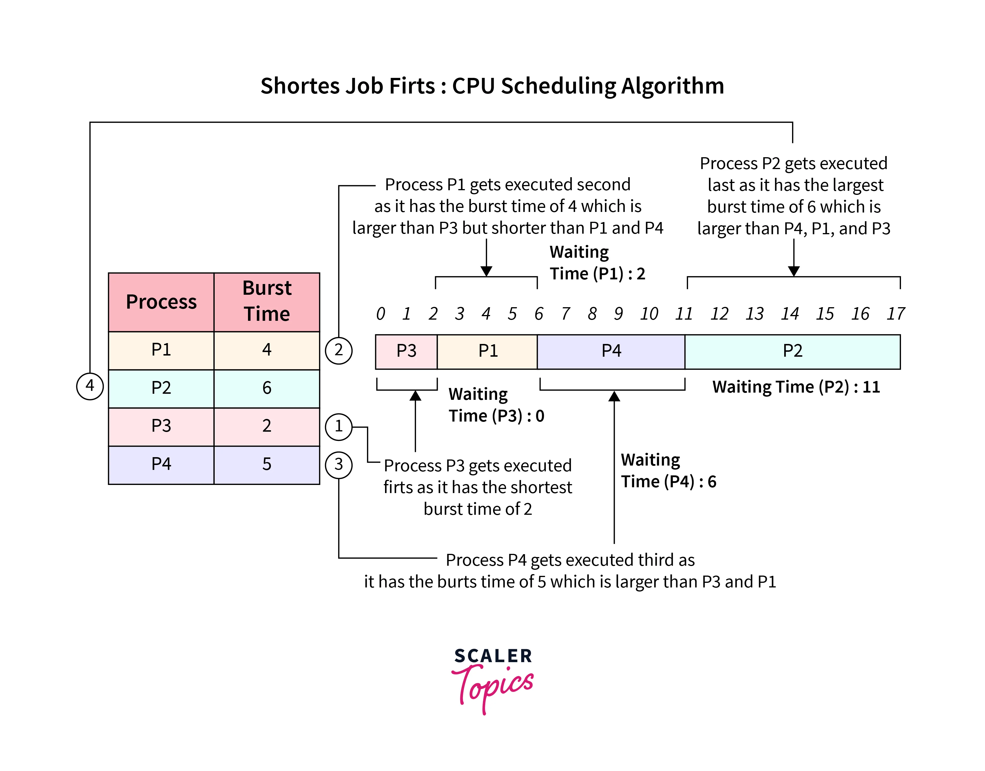
In the above example, we are taking the arrival time of each process to be . The processes are executed in ascending order according to their burst times because their arrival times are all zero. As a result, the processes are executed in the following order:
How to Compute Below Times in SJF Using a Program?
Pre-requisites:
Scaler Placement Report and Statistics
Scaler learners achieved 2.5x salary growth with average post-Scaler CTC reaching ₹23L.
Completion Time (CT)
The time in the CPU scheduling at which a process has finished running.
Formula for computing the completion time of a process:.
Turn Around Time (TAT)
The difference in time between the Completion Time of the process and the Arrival Time of the process.
Formula for computing the turnaround time of a process:.
Turn Learning into Career Growth
Waiting Time (WT)
The difference in time between Turn Around Time of the process and the Burst Time of the process.
Formula for computing the waiting time of a process:.
or
Java Program for SJF Algorithm
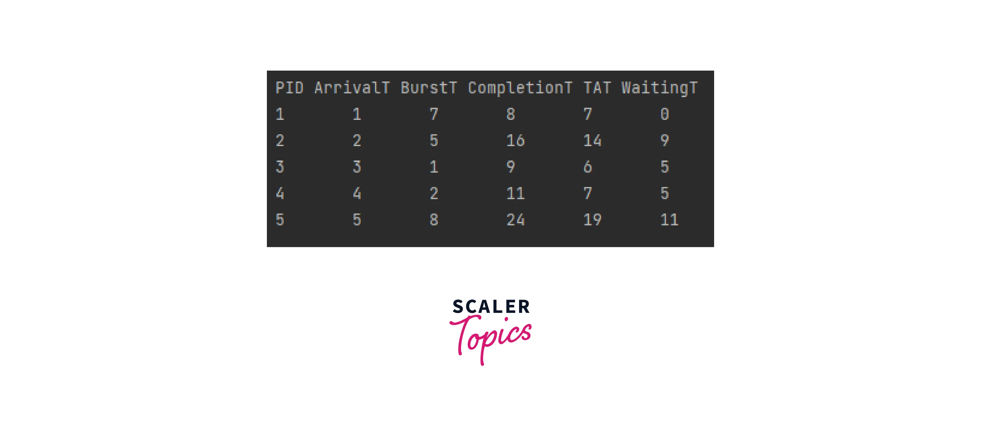
Output:
Non-Preemptive SJF
In Non-preemptive SJF scheduling, the process retains the CPU cycle once it has been assigned to the CPU until it completes its execution or is stopped.
Let's consider the below example to understand non-preemptive SJF scheduling in OS:
| Process Queue | Burst time | Arrival time |
|---|---|---|
| P1 | 2 | 2 |
| P2 | 5 | 4 |
| P3 | 3 | 0 |
| P4 | 4 | 1 |
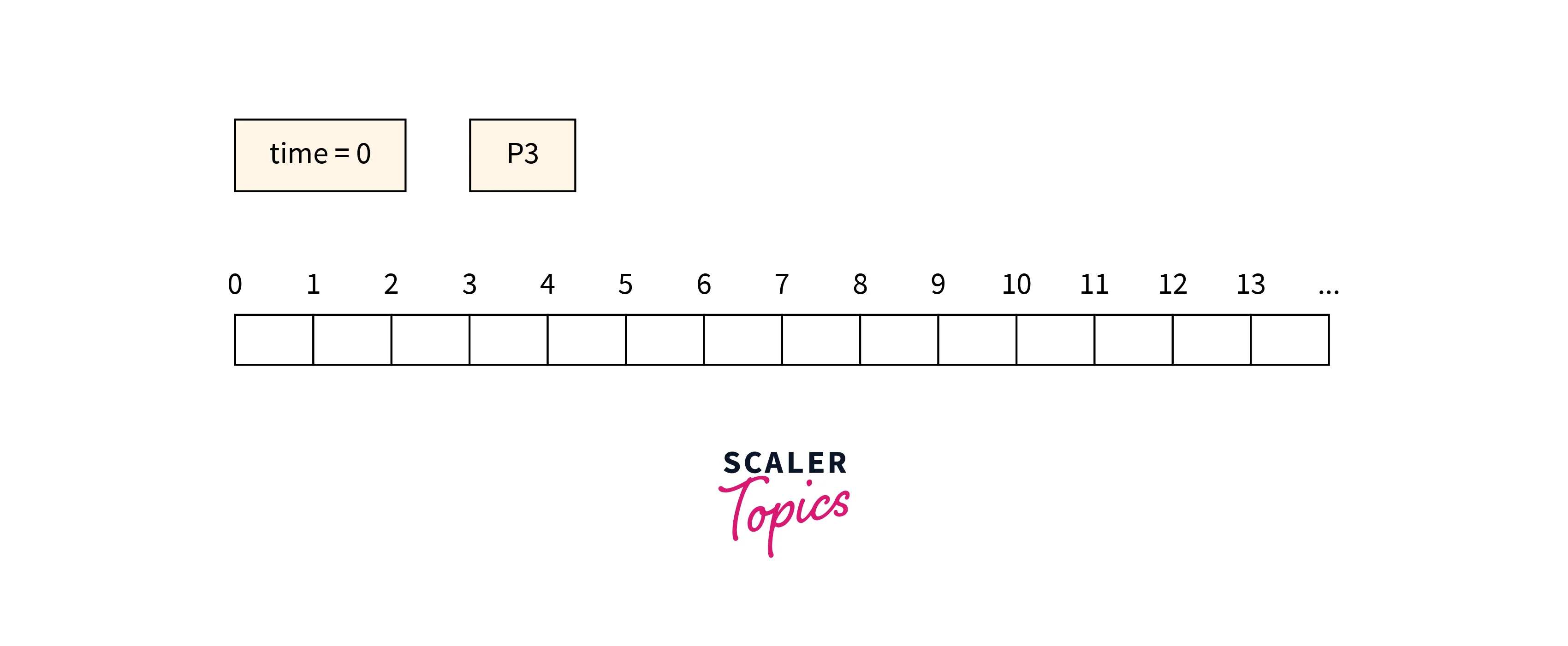
Step 0: At , Process arrives and begins execution.
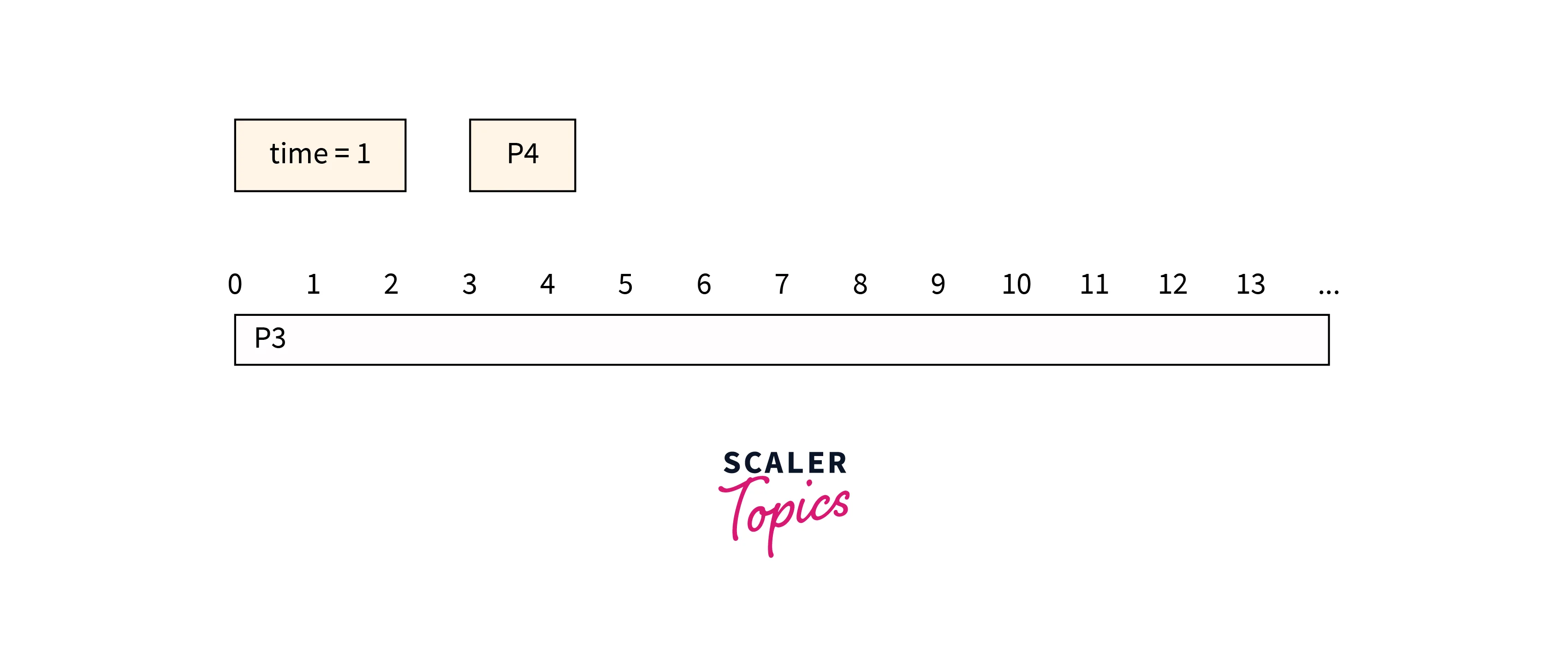
Step 1: At , process arrives. However, still needs two more units to finish. will continue to run on the CPU.
Step 2: At , process arrives and joins the queue of processes waiting for execution. will continue to run on the CPU.
Step 3: At , process execution gets completed. We compare the burst times of and . Process goes into the CPU for execution because it has a shorter burst time than Process does.

Step 4: At , process arrives and joins the queue of processes waiting for execution. process continues its execution on the CPU, and remains in the queue.
Step 5: At , process execution gets completed. We compare the burst times of and . Process goes into the CPU for execution because it has a shorter burst time than Process does.
Step 6: At , process continues execution.
Step 7: At , process completes its execution and process goes into the CPU for execution.
Step 8: At , process will complete its execution.
Step 9: Let's find out the average waiting time for a process.
Preemptive SJF
In the Preemptive SJF scheduling, jobs are inserted into the queue as they are received. The process with the least burst time starts execution, and if a job with a shorter burst time enters the queue, the current process is terminated or preempted from continuing and the shorter job is given the CPU cycle for execution.
Let's consider the below example to understand preemptive SJF scheduling in OS:
| Process Queue | Burst time | Arrival time |
|---|---|---|
| P1 | 3 | 0 |
| P2 | 1 | 4 |
| P3 | 5 | 1 |
| P4 | 4 | 2 |
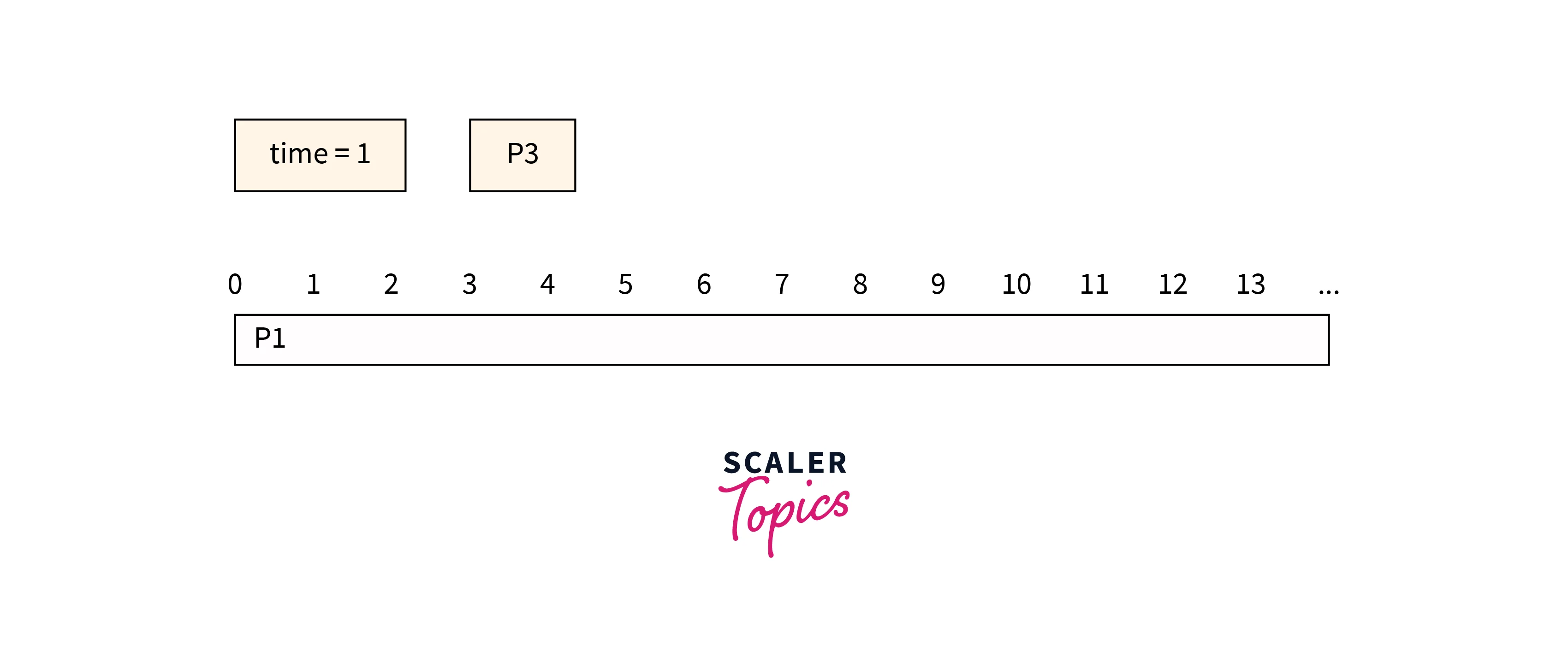
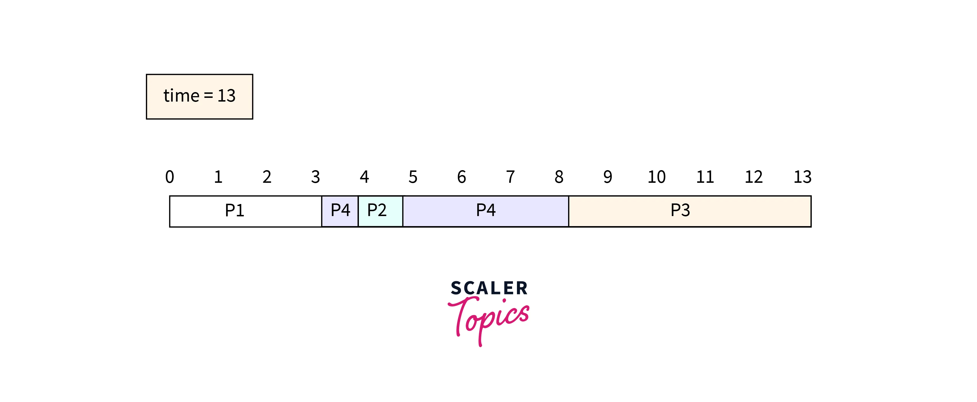
Step 0: At , process arrives and begins execution (, for , see above table).

Step 1: At , process arrives (, for ). However, has a shorter burst time, so will continue to run on the CPU, meanwhile, will go in the process queue.
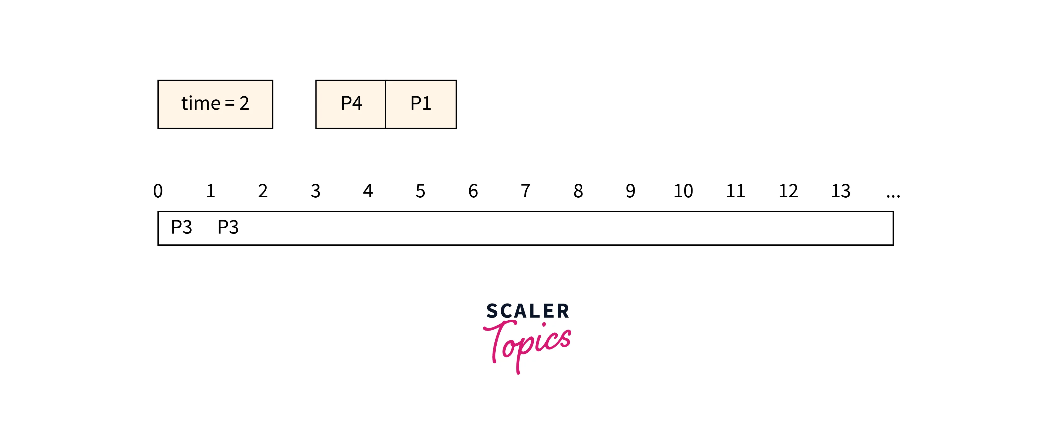
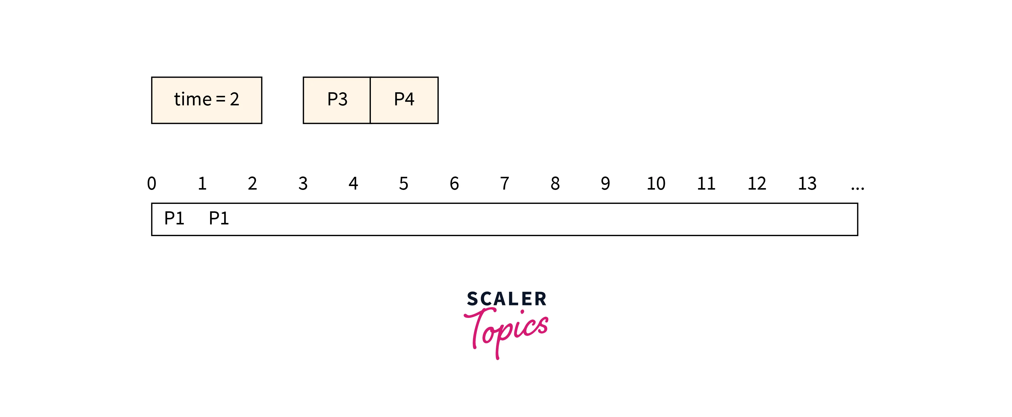
Step 2: At , process arrives (, for ) and it joins the queue of processes waiting for execution as has a shorter burst time than . will continue to run on the CPU.
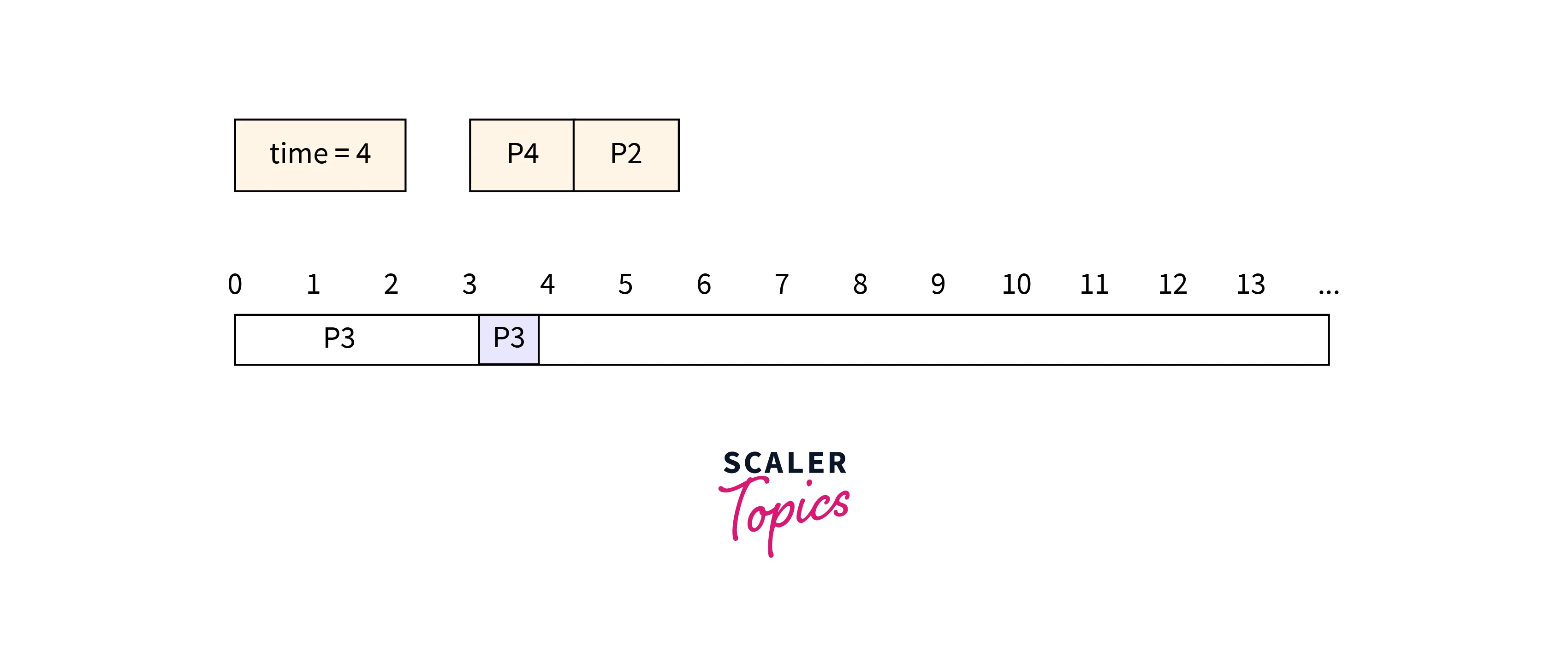
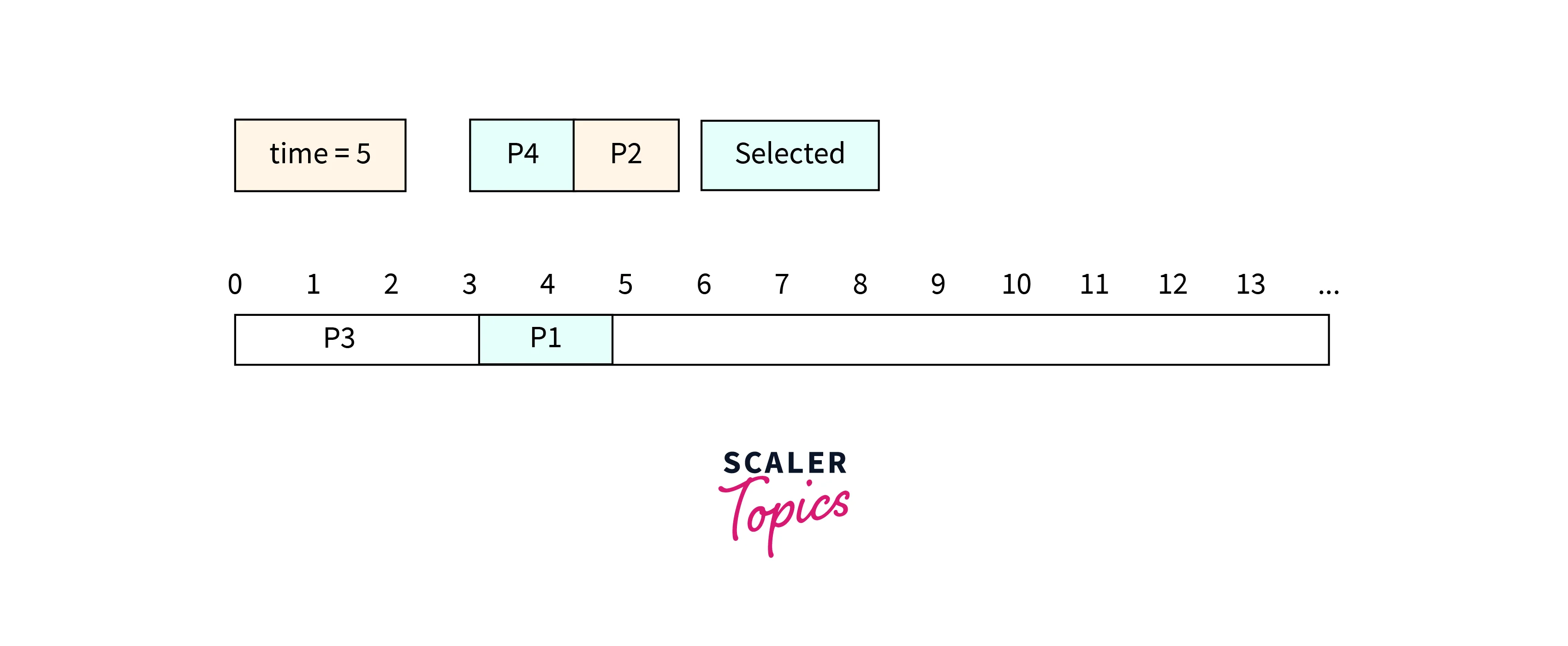
Step 3: At , process completes its execution. We compare the burst times of and . Process goes into the CPU for execution because it has a shorter burst time than Process does.
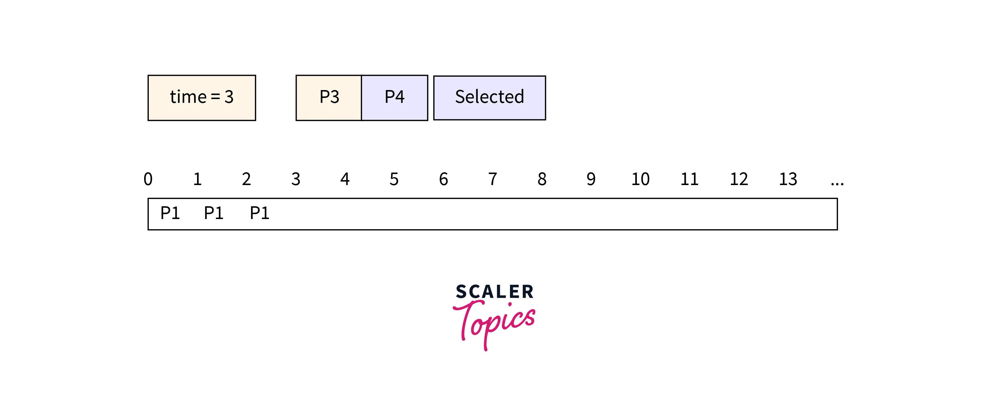
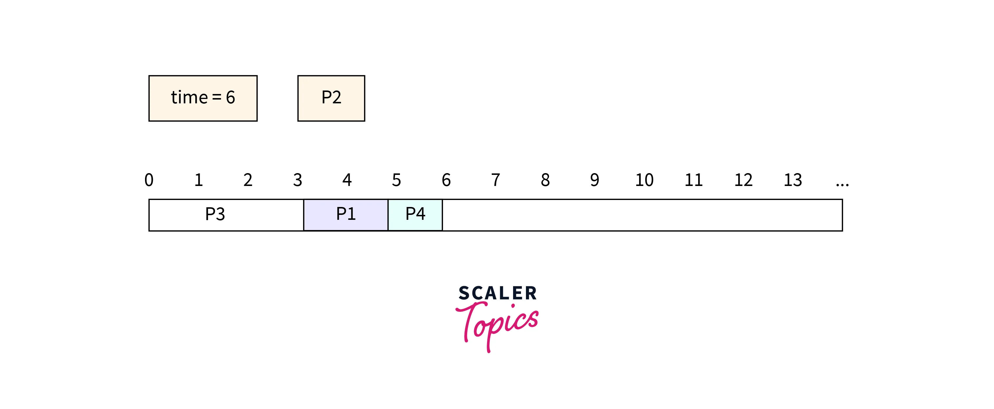
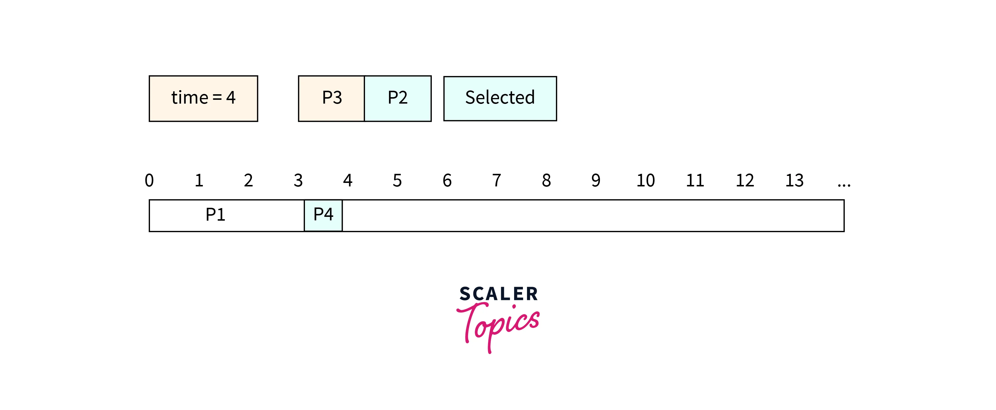
Step 4: At , process arrives with a shorter burst time (, for ) as compared to process which is currently executing. Process is terminated/preempted and starts executing.
Here, the table will look something like this:
| Process Queue | Burst time | Arrival time |
|---|---|---|
| P1 | 0 remaining | 0 |
| P2 | 1 | 4 |
| P3 | 5 | 1 |
| P4 | 3/4 remaining | 2 |
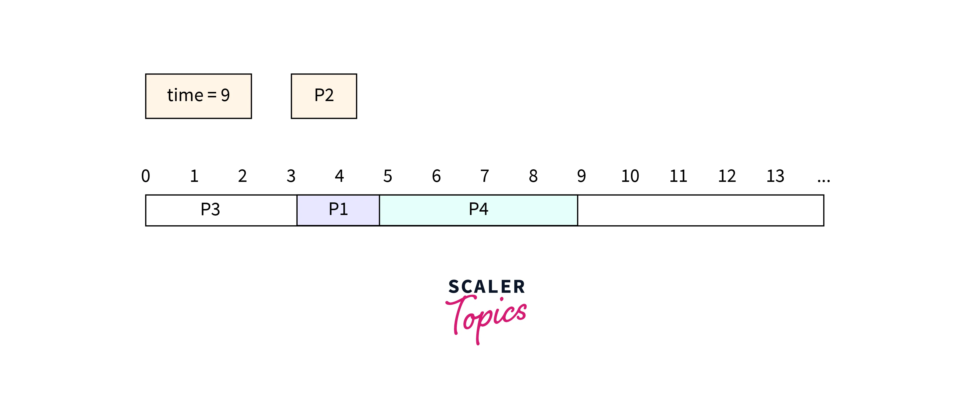
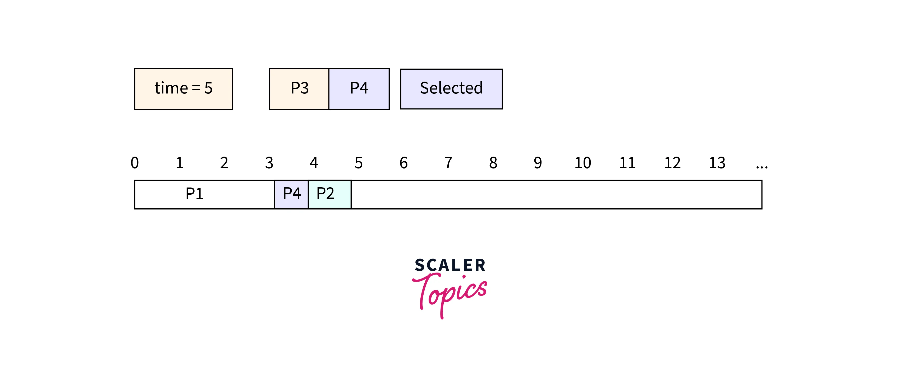
Step 5: At , process completes its execution and again starts execution as it has a shorter burst time as compared to .
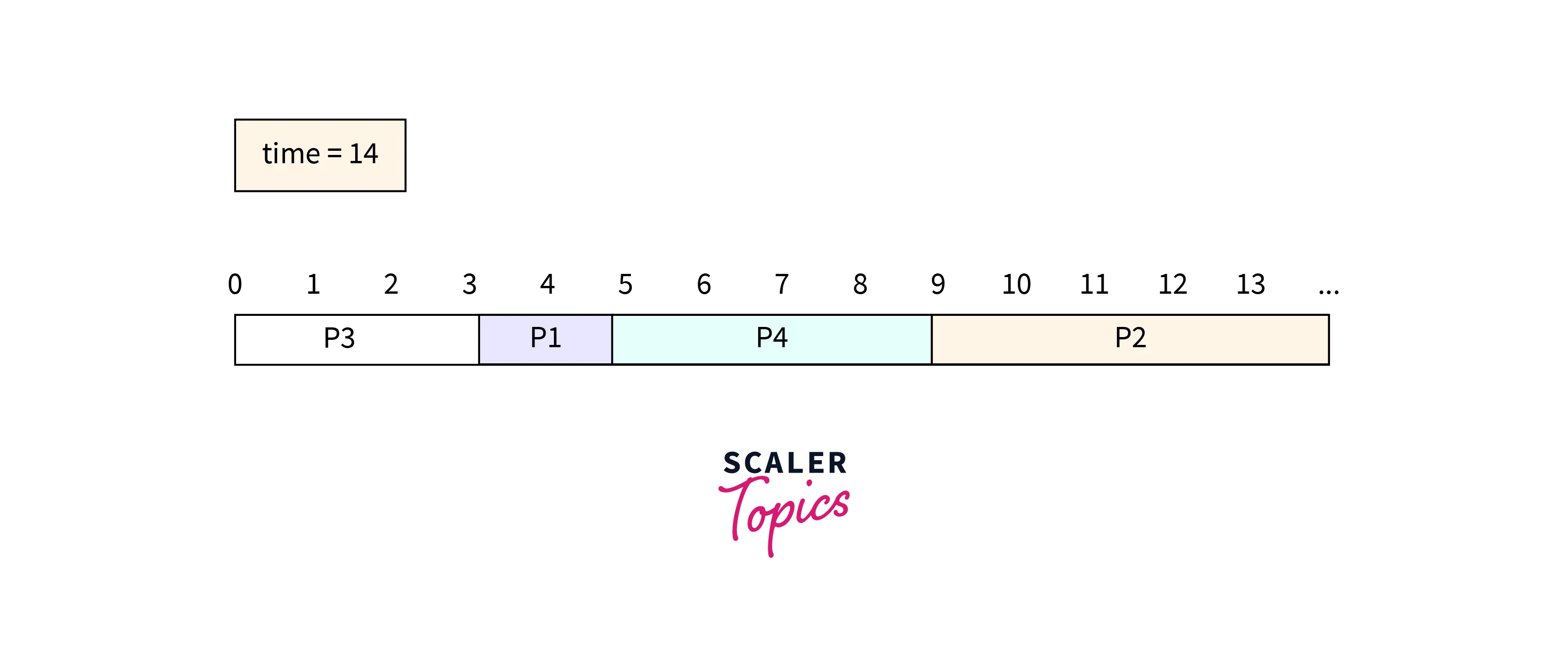
Step 6: At , process completes its execution, and starts its execution in the CPU.
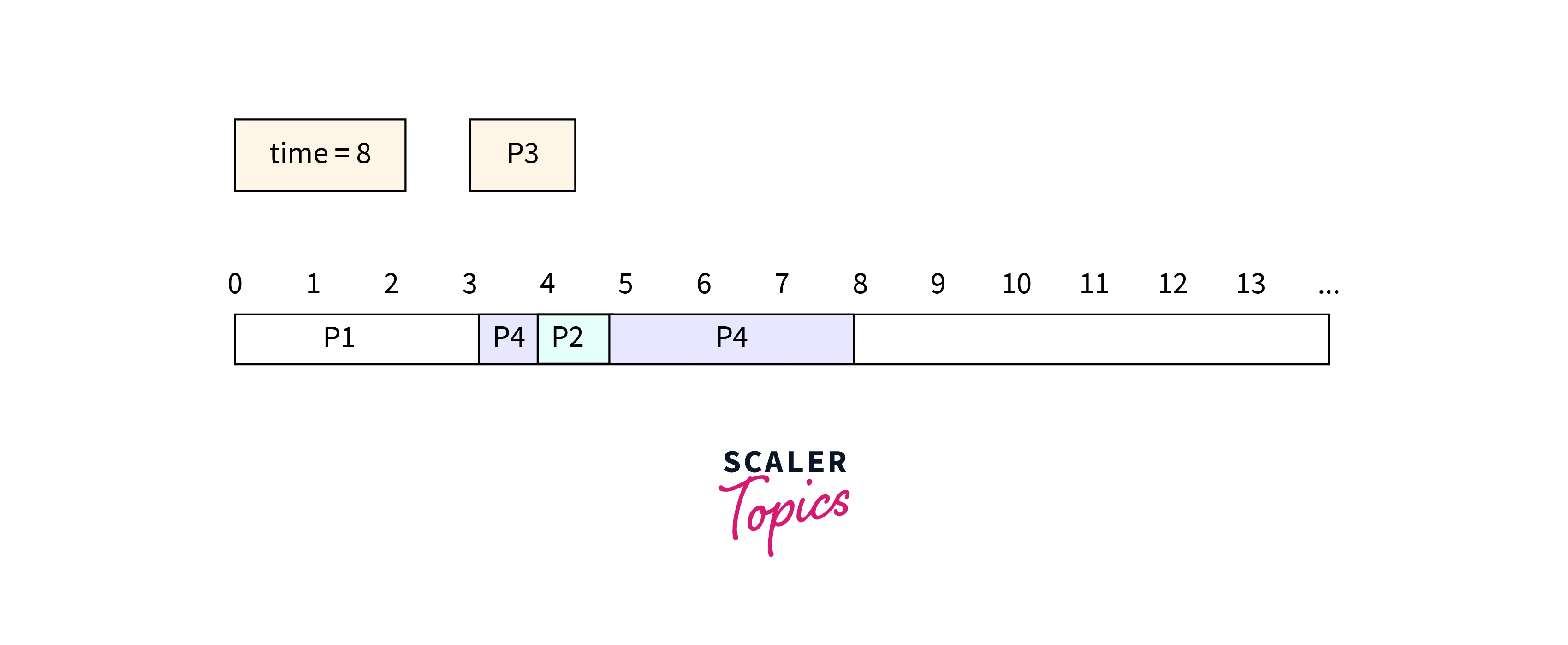
Step 7: At , process completes its execution.
Step 8: Let's find out the average waiting time for a process.
Advantages of SJF
These are some of the Advantages of the SJF algorithm:
- Shortest Job First (SJF) has a shorter average waiting time as compared to the First come first serve (FCFS) algorithm.
- SJF can be applied to long-term scheduling.
- SJF is ideal for jobs that run in batches and whose run times are known.
- SJF is probably the best concerning the average turnaround time of a process.
Disadvantages of SJF
These are some of the Disadvantages of the SJF algorithm:
- The Shortest Job First algorithm may result in a starvation problem with extremely long turnaround times.
- In SJF, job burst time must be predetermined, although it might be difficult to predict it.
- As we are unable to estimate the duration of the upcoming CPU process burst time, we cannot utilize SJF for short-term CPU scheduling.
- The processes cannot be given any priority in SJF scheduling.
Conclusion
- In the Shortest Job First algorithm, the CPU will be assigned a job with the smallest burst time first, and the processes in the queue with the shorter burst time will be received and executed by the CPU more quickly.
- There is a significant amount of decrease in the average waiting time for other processes that are left waiting to be executed.
- Usually, SJF scheduling in OS is not used with scheduling processes as it can be quite challenging to estimate the burst time required for a process.
- It is possible to use Shorted Job First Scheduling in both preemptive and non-preemptive modes. SJF scheduling in the preemptive mode is also known as the Shortest Remaining Time First (SRTF) algorithm.
- Segment Trees are used to find the minimum burst time process from all the arriving processes.