The Role of Recurrent Neural Networks in Modern Deep Learning
A recurrent neural network in deep learning is a specialized artificial neural network designed to process sequential data. Unlike standard feedforward networks, RNNs utilize an internal state (memory) to process inputs of variable lengths, making them uniquely capable of handling time-series data, natural language processing, and speech recognition.
Introduction to Recurrent Neural Networks in Deep Learning
In the broader landscape of artificial intelligence, traditional neural networks have historically operated under a critical assumption: all inputs and outputs are entirely independent of one another. While this architecture functions perfectly for isolated classification tasks—such as identifying whether an image contains a cat or a dog—it fails catastrophically when applied to sequential or contextual data. If you wish to predict the next word in a sentence, understand the sentiment of a lengthy paragraph, or forecast tomorrow's stock market prices, the network must retain contextual awareness of the data that came before it.
This is exactly where the recurrent neural network in deep learning becomes indispensable. Recurrent Neural Networks (RNNs) introduce the concept of "memory" into neural architecture. By incorporating cyclical connections, an RNN allows information to persist, passing the output of a specific node back into itself as the input for the subsequent time step. This temporal dynamic enables the network to maintain a hidden state that acts as an aggregated summary of the historical sequence. Understanding the mechanics, variants, and mathematical foundations of RNNs is a critical stepping stone for any software engineer or computer science student venturing into advanced sequence modeling, time-series forecasting, or natural language processing.
Stop learning AI in fragments—master a structured AI Engineering Course with hands-on GenAI systems with IIT Roorkee CEC Certification


AI Engineering Course Advanced Certification by IIT-Roorkee CEC
A hands on AI engineering program covering Machine Learning, Generative AI, and LLMs - designed for working professionals & delivered by IIT Roorkee in collaboration with Scaler.
Enrol Now
How a Recurrent Neural Network Works
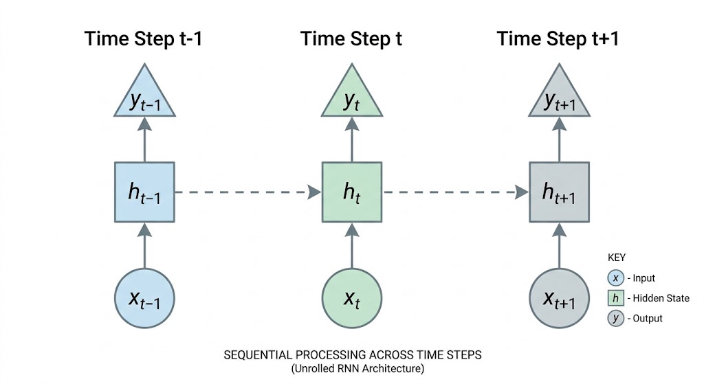
The core architectural divergence between a standard neural network and a recurrent neural network lies in the recurrent loop. In a traditional feedforward network, information flows in a single, unidirectional path from the input layer, through the hidden layers, and directly to the output layer. There is no mechanism to store intermediate representations across different data points. In an RNN, however, the hidden layer computes its activation based not only on the current input but also on the hidden state from the previous time step.
To visualize this process, computer scientists often "unroll" or "unfold" the network across time. Unrolling simply means representing the network as a sequence of identical layers, each corresponding to a specific time step in the input sequence. For an input sequence of five words, the unrolled RNN would appear as a five-layer neural network, with each layer sharing the exact same weights and biases.
Build an AI-First Career, Master the Complete Skillset
Choose from our industry-leading programs designed for career success
Modern Software and AI Engineering Program
Master full-stack development with AI integration


 +1000 more
Modern Data Science and ML with specialisation in AI
Advanced data science techniques with AI specialization
+1000 moreAdvanced AIML with Specialisation in Agentic AI
Deep dive into AIML with focus on Agentic systems
+1000 moreDevOps, Cloud & AI Platform Engineering
Build and manage AI-powered cloud infrastructure
+1000 moreAI Engineering Advanced Certification by IIT-Roorkee
Premier AI engineering certification from IIT-Roorkee

AI Forward Deployed Engineer Program
Full-stack engineering, production AI and client-facing consulting
+1000 moreThe Mathematical Formulation of Recurrence
To implement a recurrent neural network in deep learning, we must define its operations mathematically. At any given time step (t), the network receives an input vector x_t and the hidden state vector from the previous time step h_{t-1}.
The new hidden state h_t is calculated using an activation function—typically the hyperbolic tangent (tanh) or Rectified Linear Unit (ReLU)—applied to the linear combination of these two inputs. The equation is represented as:
h_t = tanh(W_hh * h_{t-1} + W_xh * x_t + b_h)
Where:
- W_hh represents the weight matrix for the hidden state.
- W_xh represents the weight matrix for the current input.
- b_h represents the bias vector for the hidden state.
Once the current hidden state h_t is computed, it can be passed forward to the next time step (t+1), and it can also be used to generate an output y_t for the current time step:
y_t = W_hy * h_t + b_y
Where:
- W_hy represents the weight matrix mapping the hidden state to the output.
- b_y represents the output bias vector.
Crucially, the weight matrices (W_hh, W_xh, W_hy) are shared across all time steps. This parameter sharing significantly reduces the total number of learnable parameters in the model, allowing the network to generalize across sequences of arbitrary length.
Backpropagation Through Time (BPTT)
Training a recurrent neural network requires a variation of the standard backpropagation algorithm known as Backpropagation Through Time (BPTT). Because the parameters are shared across all time steps in the unrolled network, the gradient of the loss function must be calculated concerning these shared weights by summing up the gradients at each individual time step.
When the network produces an output sequence, an overall loss is calculated (often Cross-Entropy Loss for classification or Mean Squared Error for regression). BPTT calculates the partial derivatives of the loss concerning the weights by applying the chain rule backward from the final time step t down to the initial time step 0. The shared weights are then updated using optimization algorithms such as Stochastic Gradient Descent (SGD) or Adam.
Recurrent Neural Network Architectures and Types
Because sequential data comes in various shapes and sizes, recurrent neural networks are highly flexible in their architectural implementation. By manipulating how inputs and outputs are mapped across time steps, engineers can tailor RNNs to solve fundamentally different classes of problems.
The versatility of an RNN is dictated by its input-to-output mapping. Below are the core structural variants utilized in modern deep learning applications.
One-to-One Architecture
The one-to-one architecture represents the simplest form of neural network configuration. It takes a single input and generates a single output. Technically, an RNN configured this way acts identical to a standard feedforward neural network because it lacks sequential processing. It is primarily used as a baseline or within specific isolated components of larger deep learning architectures. Image classification tasks typically follow this structure.
Become the Ai engineer who can design, build, and iterate real AI products, not just demos with an IIT Roorkee CEC Certification
AI Engineering Course Advanced Certification by IIT-Roorkee CEC
A hands on AI engineering program covering Machine Learning, Generative AI, and LLMs - designed for working professionals & delivered by IIT Roorkee in collaboration with Scaler.
Enrol NowOne-to-Many Architecture
In a one-to-many architecture, the network receives a single input but generates a sequence of outputs over multiple time steps. This setup is predominantly used in tasks where a static input dictates a sequential generative output. A classic example is image captioning, where a Convolutional Neural Network (CNN) extracts a single feature vector from an image, and the RNN takes that vector as an initial input to generate a sequence of words describing the image.
Many-to-One Architecture
The many-to-one architecture processes an entire sequence of inputs over multiple time steps but only generates a single output at the final time step. This structure is highly effective for sequence classification problems. For instance, in sentiment analysis, the network reads a full sentence word by word (many inputs) and ultimately outputs a single continuous value or categorical probability representing the overall sentiment (positive, negative, or neutral).
Many-to-Many Architecture
The many-to-many architecture is the most complex configuration, handling sequential inputs and sequential outputs. This architecture is typically divided into two sub-categories:
- Aligned (Synced) Sequences: The input and output lengths are identical, and an output is generated at every time step. Video frame classification or Part-of-Speech (POS) tagging heavily rely on synced sequences.
- Unaligned Sequences (Encoder-Decoder): The input sequence is processed entirely to generate a final context vector, which is then used to generate an output sequence of a different length. Machine translation algorithms (e.g., translating a five-word English sentence into a seven-word French sentence) utilize this encoder-decoder structure.
How Scaler Transformed Careers in Different Fields
Scaler learners achieved 2.5x salary growth with average post-Scaler CTC reaching ₹23L.
 Google
 Amazon
 Microsoft
 Flipkart
 Adobe1200+ more
Challenges and Limitations of Standard RNNs
While the theoretical foundation of recurrent neural networks is elegant, standard ("vanilla") RNNs suffer from severe practical limitations when dealing with long sequences. Understanding these limitations is critical for those hoping to become an ai engineer, as it directly motivates the usage of more advanced gating architectures in production environments.
The primary flaw in standard recurrent networks stems from the mathematical reality of repeatedly multiplying weight matrices and gradients across deep temporal unrollings.
The Vanishing and Exploding Gradient Problem
During Backpropagation Through Time (BPTT), the chain rule requires multiplying the gradients of the hidden states across every time step. Because the same weight matrix (W_hh) is used repeatedly, the gradient calculation involves taking the weight matrix to the power of t (the sequence length).
If the dominant eigenvalues of the weight matrix are strictly less than 1.0, the gradients exponentially decay as they propagate backward in time. By the time the gradient reaches the initial time steps of a long sequence, it becomes infinitesimally small (the vanishing gradient problem). Consequently, the network fails to update the weights associated with early inputs, completely halting the learning process for long-term dependencies.
Conversely, if the eigenvalues are greater than 1.0, the gradients grow exponentially, leading to numeric overflow and wildly unstable weight updates (the exploding gradient problem). Exploding gradients can be mitigated using a technique called gradient clipping (capping the gradient vector to a maximum norm), but vanishing gradients require architectural overhauls.
Short-Term Memory
Because of the vanishing gradient problem, standard RNNs suffer from a severely constrained context window. They possess an implicit short-term memory, meaning they can only effectively retain information from recent time steps. If a sequence is 50 steps long, the vanilla RNN will heavily weight the information from steps 45-50 but almost entirely "forget" the critical context provided in steps 1-5. This makes standard RNNs unviable for processing long documents, complex time-series data, or deeply nested code structures.
Advanced Variants: Solving RNN Limitations
To combat the inherent mathematical instability of standard recurrent architectures, researchers developed advanced gating mechanisms that regulate the flow of information through the sequence. These variants allow the network to selectively learn what to remember and what to forget over extended temporal distances.
Turn Learning into Career Growth
Long Short-Term Memory (LSTM Networks)
The most prominent and widely deployed solution to the vanishing gradient problem is Long Short-Term Memory networks, commonly referred to as LSTM networks. Introduced by Hochreiter and Schmidhuber in 1997, LSTM networks revolutionized the way a recurrent neural network in deep learning processes long-term dependencies.
Instead of a simple hidden state computed via a single tanh layer, an LSTM cell maintains an internal "cell state" (C_t). The cell state acts as an internal memory track that runs straight down the entire sequence chain with only minor linear interactions. Information is selectively added or removed from this cell state via three distinct "gates"—neural network layers equipped with a sigmoid activation function that outputs values between 0 and 1, acting as valves.
- The Forget Gate: Determines what information from the previous cell state (C_{t-1}) should be discarded. It computes: f_t = σ(W_f * [h_{t-1}, x_t] + b_f)
- The Input Gate: Determines what new information from the current input will be stored in the cell state. It creates a vector of new candidate values (C~t). i_t = σ(W_i * [h{t-1}, x_t] + b_i) C~t = tanh(W_c * [h{t-1}, x_t] + b_c)
- The Cell State Update: The old cell state is multiplied by the forget gate, and the scaled new candidate values are added: C_t = f_t * C_{t-1} + i_t * C~_t
- The Output Gate: Determines what parts of the updated cell state will be output as the new hidden state (h_t): o_t = σ(W_o * [h_{t-1}, x_t] + b_o) h_t = o_t * tanh(C_t)
By utilizing this additive update rule for the cell state, LSTM networks bypass the repeated matrix multiplication that causes gradients to vanish, allowing them to effectively bridge long temporal gaps in data.
Gated Recurrent Units (GRUs)
Introduced in 2014, the Gated Recurrent Unit (GRU) is a streamlined alternative to LSTM networks. GRUs achieve similar performance on many sequence modeling tasks but require less computational overhead. A GRU merges the cell state and hidden state into a single vector and reduces the number of gates to two:
- The Update Gate: Acts as a combination of the LSTM's forget and input gates, deciding how much past information to retain.
- The Reset Gate: Decides how much past information to forget before computing new candidate states.
Because GRUs have fewer tensor operations and parameter matrices than LSTM networks, they train significantly faster and are highly favored in resource-constrained deployment environments.
Comparing Recurrent Neural Networks to Feedforward Networks
To properly contextualize the recurrent neural network as they learn deep learning, software engineers must understand the explicit differences between an RNN and a classical Feedforward Neural Network (FFNN). Choosing the wrong architecture for a specific dataset will invariably result in catastrophic model failure.
Feedforward networks are strictly spatial in their processing capability, mapping a static tensor to an output class without any consideration for preceding inputs. Recurrent networks are inherently temporal, holding a dynamic internal state. Understanding their structural, mathematical, and practical distinctions is essential for deep learning system design. Below is a strict technical comparison mapping the key attributes of both architectures.
| Technical Feature | Feedforward Neural Network (FFNN) | Recurrent Neural Network (RNN) |
|---|---|---|
| Data Flow | Unidirectional. Data moves from input directly to output with no cycles. | Cyclical. Hidden states loop back into the network alongside new inputs. |
| Memory/State | Stateless. Operations are independent and hold no memory of previous inputs. | Stateful. Retains a hidden state vector that aggregates historical context. |
| Input Dimensionality | Fixed size. Inputs must conform to an exact, predefined tensor dimension. | Variable size. Can process sequences of varying lengths iteratively over time. |
| Parameter Sharing | None. Every fully connected layer relies on unique, independent weight matrices. | High. The same temporal weight matrices (W_hh, W_xh) are reused at every time step. |
| Backpropagation Method | Standard Backpropagation. Computes gradients linearly from output to input. | Backpropagation Through Time (BPTT). Computes gradients chronologically across unrolled steps. |
| Ideal Use Cases | Image classification, tabular data regression, standard supervised tasks. | Natural language processing, audio synthesis, time-series forecasting, machine translation. |
Practical Implementation: Building a Basic RNN in Python
In modern deep learning pipelines, standard recurrent frameworks are typically implemented using high-level libraries like PyTorch or TensorFlow. To properly grasp how the theory translates to execution, reviewing code written in a production-standard framework is essential.
In this section, we will build a fundamental Many-to-One Recurrent Neural Network using PyTorch. This architecture could be utilized for a simplified text classification or sequence prediction task.
PyTorch Code Implementation
Below is a structurally sound definition of an RNN class utilizing torch.nn.Module. Notice how we explicitly manage the dimensions of the hidden state, ensuring that the recurrent operations correctly match the sequence length and batch size defined during training.
This code illustrates the essence of an RNN: sequential inputs are iteratively processed by the nn.RNN module, and the final state representing the entire sequence's context is funneled into a standard linear classifier.
The Evolution: RNNs vs. Transformers in Modern Deep Learning
While recurrent neural networks laid the foundation for processing sequential data, the deep learning landscape has shifted radically since the introduction of the Transformer architecture in 2017.
Transformers fundamentally discard the concept of sequential temporal recurrence. Instead of parsing data chronologically step-by-step, Transformers ingest entire sequences simultaneously and rely on a mechanism called Self-Attention to determine the contextual relationship between elements, regardless of their positional distance.
This architectural shift solves the main bottleneck of RNNs: sequential computation cannot be highly parallelized. Because an RNN relies on the output of step t-1 to compute step t, it cannot leverage modern multi-core GPU architecture to process a sequence concurrently. Transformers solve this, enabling the training of massive foundation models ai architectures like GPT and BERT.
However, to claim that RNNs are obsolete would be a gross technical inaccuracy. While Transformers dominate massive-scale natural language processing, a recurrent neural network in deep learning remains incredibly relevant. Transformers demand massive memory overhead (attention scales quadratically with sequence length), making them unviable for many resource-constrained, real-time edge devices. In strict time-series forecasting, low-latency control systems, and embedded audio processing, LSTM networks and GRUs continue to be the architecture of choice due to their streamlined parameter footprint and linear scaling.
Key Applications of Recurrent Neural Networks
Due to their powerful ability to capture chronological statefulness and sequential dependencies, RNNs are still broadly utilized in specific domains explored in a data science course and artificial intelligence.
- Time-Series Forecasting: RNNs are mathematically ideal for predicting future numerical sequences based on historical data. This application spans various industries, including stock market price prediction, epidemiological modeling, and smart grid energy demand forecasting.
- Predictive Maintenance: In industrial IoT environments, recurrent models continuously ingest sensor data (vibration, temperature, pressure) from heavy machinery to predict mechanical failures before they occur, relying heavily on temporal pattern recognition.
- Speech Recognition and Generation: Converting continuous audio waveforms into text requires interpreting sequential audio frames. Recurrent models are deeply embedded in acoustic modeling pipelines to manage the temporal nature of human speech.
- Natural Language Processing (Specialized): While massive LLMs use Transformers, smaller-scale NLP tasks—such as automated text summarization on local devices, intent classification in fast-response chatbots, and predictive typing on mobile keyboards—often utilize lightweight LSTM networks to minimize battery consumption and latency.
FAQs
What is the fundamental difference between an RNN and an LSTM? An RNN is the general category of neural networks that utilizes recurrent connections to process sequential data. However, a standard RNN suffers from short-term memory due to the vanishing gradient problem. An LSTM is a highly specialized variant of an RNN that utilizes internal memory tracks (cell states) and gating mechanisms to effectively retain information over much longer sequences.
Why do gradients vanish in standard RNNs? Gradients vanish because Backpropagation Through Time (BPTT) requires the repeated multiplication of the same hidden state weight matrix across every time step. If the matrix values are less than one, applying the chain rule continuously over long sequences causes the gradient values to shrink exponentially until they approach zero.
Can an RNN process inputs of varying lengths in the same batch? Yes, but it requires data preprocessing techniques. Since neural networks require fixed tensor dimensions for batch matrix multiplication, sequences of varying lengths must be padded with zeroes to match the longest sequence in the batch. Advanced frameworks like PyTorch utilize utility functions like pack_padded_sequence to ensure the RNN ignores the padded elements during computation, optimizing efficiency.
Why is an RNN considered stateful? An RNN is stateful because it continuously maintains and updates a hidden state vector. This vector acts as an aggregated mathematical memory of all the sequential inputs the network has processed up to the current time step, allowing past data points to influence future predictions.