What is Convolutional Neural Network? Complete Guide
A Convolutional Neural Network (CNN) is a specialized type of artificial neural network designed to process and analyze structured grid data, primarily images. It utilizes mathematical convolution operations instead of general matrix multiplication in at least one of its layers to automatically extract spatial hierarchies of features.
Computer vision has undergone a massive paradigm shift over the last decade, transitioning from manual feature engineering algorithms—like Haar Cascades and Scale-Invariant Feature Transform (SIFT)—to automated, deep learning-based approaches. At the absolute core of this transformation is the Convolutional Neural Network. By mimicking the connectivity pattern between neurons in the human visual cortex, CNNs have established a new state-of-the-art benchmark for image classification, object detection, and autonomous navigation.
This guide provides a comprehensive architectural breakdown of CNNs, detailing their mathematical foundations, layer configurations, and practical implementations.
What is Convolutional Neural Network?
A Convolutional Neural Network (often abbreviated as CNN or ConvNet) is a deep learning architecture explicitly engineered to process data that has a known, grid-like topology. The most common application of this is 2D image data, which consists of a grid of pixels. However, CNNs are also highly effective on 1D sequential data (like audio signals or time-series data) and 3D volumetric data (like MRI scans).
Traditional neural networks struggle with high-dimensional input data. If you were to pass a high-resolution image into a standard multi-layer perceptron (MLP), the number of required parameters would be astronomically high, leading to rapid overfitting and unmanageable computational costs. Furthermore, MLPs flatten the image into a one-dimensional array before processing, permanently destroying the critical spatial and topological relationships between neighboring pixels.
To solve this, CNNs introduce three core architectural concepts: local receptive fields, shared weights, and spatial subsampling. Instead of connecting every input neuron to every hidden neuron, CNNs use small, localized filters (kernels) that slide across the input data. This ensures that the network preserves spatial relationships, recognizing an edge, curve, or texture regardless of where it appears in the visual field.
Stop learning AI in fragments—master a structured AI Engineering Course with hands-on GenAI systems with IIT Roorkee CEC Certification
AI Engineering Course Advanced Certification by IIT-Roorkee CEC
A hands on AI engineering program covering Machine Learning, Generative AI, and LLMs - designed for working professionals & delivered by IIT Roorkee in collaboration with Scaler.
Enrol Now
Scaler Placement Report and Statistics
Scaler learners achieved 2.5x salary growth with average post-Scaler CTC reaching ₹23L.
How Do CNNs Work?
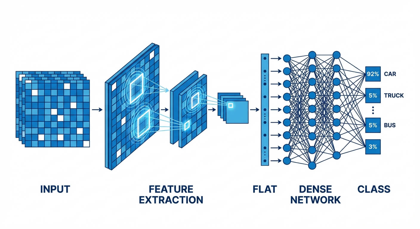
Understanding how do CNNs work requires dissecting the hierarchical approach they take to feature extraction. Rather than trying to understand an entire image at once, a CNN builds a representation of the image layer by layer, moving from granular, low-level features to complex, high-level semantic structures.
When an image is fed into a CNN, the network processes it through a series of specialized layers. In the initial layers, the network acts as a collection of low-level feature detectors. The filters in these early layers learn to identify simple geometric patterns: horizontal lines, vertical edges, color gradients, and sharp corners.
As the data propagates deeper into the network, the outputs of these early layers (feature maps) become the inputs for subsequent layers. The middle layers combine these basic edges to detect shapes, such as circles, squares, or specific textures. By the time the data reaches the final convolutional layers, the network is assembling these shapes into recognizable high-level objects—like a human face, a dog's snout, or a car tire. Finally, this rich spatial representation is flattened and passed into fully connected layers to map the extracted features to specific class probabilities.
Core Building Blocks of a CNN Architecture
The architecture of a Convolutional Neural Network is not a monolith; it is a modular sequence of specific mathematical operations arranged into layers. A standard CNN primarily consists of three types of layers: Convolutional Layers, Pooling Layers, and Fully Connected Layers.
The Convolutional Layer
The Convolutional Layer is the core building block of a CNN, responsible for the vast majority of the network's computational heavy lifting. Its primary purpose is to extract features from the input data.
Instead of connecting to all pixels, each neuron in a convolutional layer connects only to a small, localized region of the input volume. This is achieved using a "filter" or "kernel"—a small matrix of weights (for example, a 3x3 or 5x5 matrix). During the forward pass, this filter slides (or "convolves") across the width and height of the input volume. At every spatial position, the network computes the dot product between the entries of the filter and the corresponding input pixels.
This process produces a 2D activation map (or feature map) that gives the responses of that filter at every spatial position. If a filter is trained to detect horizontal edges, its feature map will light up with high activation values wherever a horizontal edge exists in the original image.
Key parameters in a convolutional layer include:
- Kernel Size: The spatial dimensions of the filter (e.g., 3x3).
- Stride: The number of pixels by which the filter moves across the input matrix. A stride of 1 means the filter moves one pixel at a time. A larger stride produces a smaller output feature map.
- Padding: As the filter slides across the image, the spatial dimensions of the output shrink. To preserve the original spatial dimensions, networks use "Zero-Padding" (adding a border of zeros around the input image).
- Valid Padding: No padding is applied. The feature map shrinks.
- Same Padding: Padding is applied so the output feature map has the same spatial dimensions as the input.
Activation Functions: Introducing Non-Linearity
If a CNN only utilized convolutional layers, it would merely be computing linear transformations. Because real-world data is highly non-linear, the network must inject non-linearity to learn complex patterns.
Immediately following a convolution operation, the output is passed through an activation function. The most ubiquitous activation function in modern CNNs is the Rectified Linear Unit (ReLU).
The mathematical function for ReLU is remarkably simple: f(x) = max(0, x)
ReLU iterates through the feature map and replaces all negative values with zero, while leaving positive values unchanged. This operation is computationally efficient and fundamentally mitigates the vanishing gradient problem, allowing deep networks to train much faster and more reliably than older activation functions like Sigmoid or Tanh.
The Pooling Layer (Downsampling)
It is common practice to periodically insert a Pooling layer between successive Convolutional layers in a CNN architecture. Its function is to progressively reduce the spatial size (width and height) of the representation, reducing the number of parameters and computation in the network, and thereby controlling overfitting.
Pooling operates independently on every depth slice of the input and resizes it spatially. The two most common types are:
- Max Pooling: Slides a window (typically 2x2 with a stride of 2) over the feature map and outputs the maximum value within that window. This is the most popular technique because it retains the most prominent features (highest activations) while aggressively reducing spatial dimensions.
- Average Pooling: Calculates the average value of the elements within the window. While useful in specific architectural endpoints, it is less common in intermediate layers than Max Pooling.
By downsampling the data, pooling layers create spatial invariance. This means that if a distinct feature (like a cat's ear) shifts a few pixels to the left or right in the input image, the max-pooling layer will still capture the high activation, making the network robust to slight translations and distortions.
Transform Your Career
Choose from our industry-leading programs designed for career success
Modern Software and AI Engineering Program
Master full-stack development with AI integration

Modern Data Science and ML with specialisation in AI
Advanced data science techniques with AI specialization
Advanced AIML with Specialisation in Agentic AI
Deep dive into AIML with focus on Agentic systems
DevOps, Cloud & AI Platform Engineering
Build and manage AI-powered cloud infrastructure
AI Engineering Advanced Certification by IIT-Roorkee
Premier AI engineering certification from IIT-Roorkee
The Fully Connected (FC) Layer
After the input image has passed through multiple sequences of convolution, ReLU, and pooling, the network has successfully extracted the high-level features and reduced the spatial dimensions. However, this output is still in the form of 3D feature maps.
To perform the final classification, these 3D feature maps are "flattened" into a single 1D vector. This vector is then fed into one or more Fully Connected layers (identical to those in a standard artificial neural network). Every neuron in the FC layer is connected to every neuron in the preceding layer.
The final Fully Connected layer typically outputs an array of values corresponding to the number of classes the network is trying to predict. For a multi-class classification problem, this raw output is passed through a Softmax activation function, which normalizes the values into a discrete probability distribution (where all probabilities sum to 1).
Mathematical Foundation of Convolution
To truly master Convolutional Neural Networks, an engineer must understand the deterministic math governing the spatial transformations at each layer.
Consider an input image matrix I and a smaller filter matrix K (the kernel). The convolution operation (often denoted by an asterisk *) in a discrete 2D space is defined as:
S(i, j) = (I * K)(i, j) = Σ_m Σ_n I(i + m, j + n) K(m, n)
Here, the network calculates the sum of element-wise multiplications between the kernel and the overlapping region of the input image. A bias term b is subsequently added to this sum before it is passed to the activation function. Master structured AI Engineering + GenAI hands-on, earn IIT Roorkee CEC Certification at ₹40,000
Calculating Output Dimensions
A critical skill in deep learning engineering is calculating the exact shape of your tensors as they flow through the network. If your tensor dimensions mismatch, your code will fail to compile.
You can calculate the spatial dimension of an output feature map using the following formula:
O = [(W - K + 2P) / S] + 1
Where:
- O = Output dimension (Width or Height)
- W = Input dimension (Width or Height)
- K = Spatial size of the Kernel/Filter
- P = Amount of Zero Padding applied to the borders
- S = Stride length
Example Calculation: Suppose you have an input image of size 227x227x3 (Width=227, Height=227, Channels=3). You apply a Convolutional layer with 96 filters. Each filter has a size of 11x11 (K=11), a stride of 4 (S=4), and no padding (P=0).
Applying the formula to find the output width/height: O = [(227 - 11 + (2 * 0)) / 4] + 1 O = [216 / 4] + 1 O = 54 + 1 O = 55
Since we used 96 filters, the final output tensor shape from this specific convolutional layer will be 55x55x96.
Convolutional Neural Networks vs Fully-Connected Feedforward Neural Networks
It is vital to delineate why we cannot simply use standard multi-layer perceptrons (Feedforward Neural Networks) for complex computer vision tasks. While both architectures process inputs via weighted connections and use backpropagation to update those weights, their treatment of spatial data differs radically.
| Feature | Convolutional Neural Network (CNN) | Feedforward Neural Network (FNN) |
|---|---|---|
| Data Structure Handling | Processes multidimensional grid data (2D/3D matrices) directly, preserving spatial structure. | Requires data to be flattened into a 1D vector, permanently destroying 2D spatial relationships. |
| Weight Sharing | Uses shared kernel weights across the entire image. A feature learned in one area is recognized everywhere. | No weight sharing. Every input node has a unique, independent weight connection to every hidden node. |
| Parameter Efficiency | Highly efficient. The number of parameters depends on the filter size and number of filters, not input size. | Highly inefficient for images. High-resolution inputs lead to an explosion in parameter count. |
| Translation Invariance | Naturally translation invariant due to sliding filters and max-pooling operations. | Highly sensitive to translation. If an object moves one pixel, the FNN treats it as a completely new pattern. |
| Primary Use Case | Computer Vision, Image Classification, Video Processing, Medical Imaging. | Tabular Data, Basic Regression, simple classification tasks with non-spatial features. |
Prominent CNN Architectures (Case Studies)
The evolution of Convolutional Neural Networks can be traced through several landmark architectures that won the prestigious ImageNet Large Scale Visual Recognition Challenge (ILSVRC). Studying these models provides insight into how CNN design principles have evolved.
LeNet-5 (1998)
Developed by Yann LeCun, LeNet-5 was one of the first successful applications of CNNs. Designed primarily to recognize handwritten digits (the MNIST dataset) for bank check processing, it established the foundational pattern of alternating convolutional layers and average pooling layers, ending with fully connected layers.
Transform Your Career
Choose from our industry-leading programs designed for career success
Modern Software and AI Engineering Program
Master full-stack development with AI integration
Modern Data Science and ML with specialisation in AI
Advanced data science techniques with AI specialization
Advanced AIML with Specialisation in Agentic AI
Deep dive into AIML with focus on Agentic systems
DevOps, Cloud & AI Platform Engineering
Build and manage AI-powered cloud infrastructure
AI Engineering Advanced Certification by IIT-Roorkee
Premier AI engineering certification from IIT-Roorkee
AlexNet (2012)
AlexNet, created by Alex Krizhevsky, Ilya Sutskever, and Geoffrey Hinton, is arguably the most famous CNN. It decimated its competitors in the 2012 ImageNet challenge, proving that deep learning was viable. AlexNet popularized the use of the ReLU activation function to solve the vanishing gradient problem and utilized Dropout to prevent overfitting. Furthermore, it proved that CNNs could be effectively trained on GPUs to handle massive datasets.
Scaler Placement Report and Statistics
Scaler learners achieved 2.5x salary growth with average post-Scaler CTC reaching ₹23L.
VGG-16 (2014)
Developed by the Visual Geometry Group at Oxford, VGG-16 simplified network design rules. Instead of using large filters (like the 11x11 filters in AlexNet), VGG-16 exclusively used very small 3x3 filters with a stride of 1, stacked deeply. The authors proved that stacking multiple small filters has the same effective receptive field as one large filter, but requires fewer parameters and introduces more non-linearities, leading to deeper and more accurate networks.
ResNet (Residual Networks) (2015)
As researchers tried to build deeper networks (e.g., 50 or 100 layers) to achieve higher accuracy, they encountered the "degradation problem"—adding more layers actually caused accuracy to plummet due to gradients vanishing during backpropagation. ResNet solved this by introducing "Skip Connections" (or shortcut connections). These connections allow the gradient to bypass layers, fundamentally changing how deep networks are trained and allowing models to scale to hundreds of layers.
Building a CNN for Image Classification: Code Example
To practically illustrate these concepts, below is a standard implementation of a Convolutional Neural Network using Python and the Keras/TensorFlow library. This architecture is suitable for a standard image classification task like CIFAR-10.
Applications of Convolutional Neural Networks
The inherent ability of CNNs to detect hierarchical patterns has led to their adoption across dozens of industries, far beyond simple image categorization.
Object Detection and Localization
While standard classification simply answers "What is in this image?", object detection answers "What is in this image, and exactly where is it located?". Architectures based on CNNs, such as YOLO (You Only Look Once) and Faster R-CNN, draw precise bounding boxes around multiple objects in a single frame. This is the foundational technology powering the perception systems of autonomous vehicles, allowing them to differentiate between pedestrians, stop signs, and other cars in real-time.
Semantic Segmentation
In semantic segmentation, the network does not just draw a bounding box; it classifies every single pixel in the image. This means the CNN outputs a highly detailed mask separating the foreground from the background. Specialized CNN architectures like U-Net are heavily utilized for this task, particularly in medical imaging, where they are used to segment brain tumors or trace blood vessels in MRI and CT scans with sub-millimeter precision.
Facial Recognition Systems
CNNs are the driving force behind modern biometric security. Networks trained on millions of human faces learn to map facial features into a highly compact, multi-dimensional vector space. When you unlock your smartphone with your face, a CNN processes your live image, generates a feature vector, and compares the mathematical distance between that vector and the stored vector of your registered face to authenticate you.
Natural Language Processing (NLP)
While Transformers and Recurrent Neural Networks (RNNs) traditionally dominate textual data, 1D Convolutional Neural Networks are highly effective at certain NLP tasks. By treating a sentence as a 1D sequence of words (or characters), 1D CNNs can slide text-based filters across a document to detect strong n-gram patterns, making them incredibly fast and efficient for tasks like sentiment analysis and spam detection.
FAQs
Why do we need padding in Convolutional Neural Networks?
Padding is primarily used to prevent the rapid spatial shrinking of feature maps as they pass through multiple convolutional layers. Without padding, pixels on the edges of an image are only processed by the kernel once, whereas central pixels are processed multiple times. Padding the borders with zeros ensures edge pixels are weighted appropriately and allows engineers to design much deeper networks without the spatial dimensions collapsing to zero prematurely.
What is the difference between Max Pooling and Average Pooling?
Max Pooling selects the single highest value from the kernel window, effectively keeping only the most prominent, highly-activated feature in that region while discarding the rest. Average Pooling calculates the mean of all values in the window, preserving the overall background context but potentially diluting the sharpness of strong features. Max pooling is generally preferred in intermediate layers for image classification because identifying the presence of a strong feature (like an edge) is more important than knowing its precise location.
Become the Ai engineer who can design, build, and iterate real AI products, not just demos with an IIT Roorkee CEC Certification
AI Engineering Course Advanced Certification by IIT-Roorkee CEC
A hands on AI engineering program covering Machine Learning, Generative AI, and LLMs - designed for working professionals & delivered by IIT Roorkee in collaboration with Scaler.
Enrol NowHow does a CNN handle colored (RGB) images?
A standard grayscale image is represented as a 2D matrix (Width x Height). A colored image is represented as a 3D tensor (Width x Height x Channels), where the 3 channels represent Red, Green, and Blue pixel intensities. When processing an RGB image, the convolutional filter is also three-dimensional (e.g., 3x3x3). The kernel calculates the dot product across all three color channels simultaneously, summing them together (along with the bias) to produce a single 2D feature map.
What causes overfitting in Convolutional Neural Networks, and how is it prevented?
Overfitting occurs when a CNN is overly complex (containing millions of parameters) and memorizes the training data's exact noise and anomalies rather than learning generalizable patterns. When this happens, the model performs exceptionally well on training data but poorly on unseen test data. Engineers prevent overfitting in CNNs by utilizing techniques such as Data Augmentation (artificially rotating, flipping, or scaling training images), Dropout (randomly deactivating a percentage of neurons during training to force the network to learn redundant representations), and L2 Weight Regularization.