A Deep Dive into Recurrent Neural Networks: Mastering Sequence Data
What is recurrent neural network? A recurrent neural network (RNN) is a specialized class of artificial neural networks designed to process sequential data. Unlike traditional feedforward networks or the random forest algorithm in machine learning, RNNs utilize internal memory states and feedback loops, allowing them to retain information from prior inputs to inform current and future sequential predictions.
Introduction to the Recurrent Neural Network
The recurrent neural network represents a monumental shift in how machine learning models—often studied in a comprehensive data science course—understand temporal dynamics and sequential data. Standard feedforward networks operate on a fundamental assumption: all inputs and outputs are strictly independent of one another. However, this assumption collapses when processing sequential streams such as natural language, time-series financial data, or audio signals. In these domains, the context provided by preceding data points is mathematically strictly required to interpret the current input accurately.
To solve this dependency issue, recurrent neural networks introduce the concept of "parameter sharing" across a temporal dimension. By feeding the output of a hidden layer from the previous time step back into the same hidden layer for the current time step, the network maintains a highly dynamic internal state—often referred to as a "memory." This foundational architecture forces the network to learn not just from the immediate input vector, but from an aggregated historical context vector. This capability forms the backbone of modern sequential modeling, driving the initial architectures behind machine translation, speech recognition, and complex forecasting systems.
Stop learning AI in fragments—master a structured AI Engineering Course with hands-on GenAI systems with IIT Roorkee CEC Certification
AI Engineering Course Advanced Certification by IIT-Roorkee CEC
A hands on AI engineering program covering Machine Learning, Generative AI, and LLMs - designed for working professionals & delivered by IIT Roorkee in collaboration with Scaler.
Enrol Now
Feedforward Neural Networks vs. Recurrent Neural Networks
To understand the structural advantages of a recurrent neural network, it is essential to compare it directly to a standard Artificial Neural Network (ANN) or Feedforward Network.
| Feature | Feedforward Neural Network | Recurrent Neural Network |
|---|---|---|
| Input Structure | Fixed-size inputs only. | Variable-length sequential inputs. |
| Memory Mechanism | No internal memory. Outputs depend only on the current input. | Hidden states act as memory, retaining context from previous inputs. |
| Information Flow | Unidirectional (Input → Hidden → Output). | Cyclical (Hidden states loop back into themselves across time steps). |
| Parameter Sharing | Weights are independent at every layer. | Weights are shared across all time steps in the sequence. |
| Primary Use Cases | Image classification, tabular data, cross-sectional prediction. | Natural language processing, time-series analysis, speech recognition. |
Architectural Fundamentals of an RNN
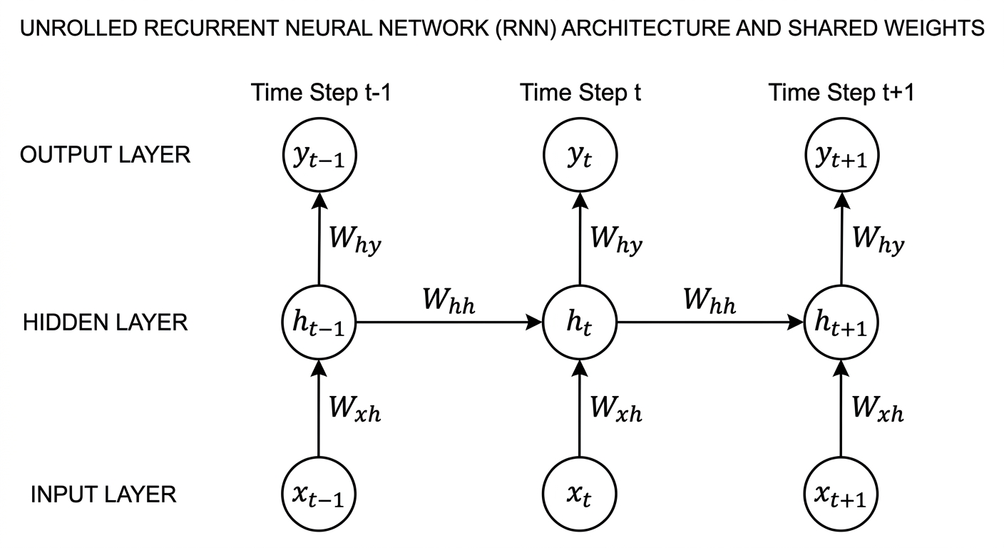
The core architecture of a recurrent neural network relies on unrolling a computational graph across time. Rather than having a purely static sequence of distinct layers, an RNN consists of a repeating cell that processes data recursively. To fully grasp this, you must understand the mathematical formulations that govern the forward propagation through an RNN cell. The network operates on three primary weight matrices: the weights connecting the input to the hidden layer, the weights connecting the previous hidden state to the current hidden state, and the weights connecting the hidden state to the output.
By keeping these weight matrices identical across all time steps (parameter sharing), the network avoids exploding in computational size while forcing the optimization algorithm to find generalized rules for transitioning states regardless of absolute time. This design is highly elegant but requires specific mathematical operations—typically involving the hyperbolic tangent (tanh) activation function to regulate the state values between -1 and 1, ensuring the memory vector does not arbitrarily balloon during long sequential reads.
Transform Your Career
Choose from our industry-leading programs designed for career success
Modern Software and AI Engineering Program
Master full-stack development with AI integration

Modern Data Science and ML with specialisation in AI
Advanced data science techniques with AI specialization
Advanced AIML with Specialisation in Agentic AI
Deep dive into AIML with focus on Agentic systems
DevOps, Cloud & AI Platform Engineering
Build and manage AI-powered cloud infrastructure
AI Engineering Advanced Certification by IIT-Roorkee
Premier AI engineering certification from IIT-Roorkee
Forward Propagation and State Formulation
In a standard recurrent neural network, the forward pass at a specific time step (t) is calculated using the input at that time step, x(t), and the hidden state from the previous time step, h(t-1).
-
Hidden State Calculation: The hidden state h(t) serves as the memory of the network. It is computed as: h(t) = tanh(W_hx * x(t) + W_hh * h(t-1) + b_h)
Where:
- W_hx represents the weight matrix mapping the input vector to the hidden state.
- W_hh represents the weight matrix mapping the previous hidden state to the current hidden state.
- b_h represents the bias vector for the hidden state computation.
- tanh is the non-linear activation function.
-
Output Calculation: The output y(t) at the current time step is derived directly from the current hidden state: y(t) = f(W_yh * h(t) + b_y)
Where:
- W_yh represents the weight matrix mapping the hidden state to the output.
- b_y represents the output bias vector.
- f represents the output activation function (e.g., Softmax for classification).
Training Recurrent Neural Networks: Backpropagation Through Time (BPTT)
Training a recurrent neural network requires a fundamentally different approach than training standard feedforward networks due to the temporal dependencies inherent in the architecture. Because the hidden state at any given time step relies on the hidden state of the previous time step, computing gradients requires calculating the derivative of the loss function not just with respect to the current state, but chaining it backwards across all previous states in the sequence. This methodology is formally known as Backpropagation Through Time (BPTT).
BPTT essentially treats the recurrent network as a deep feedforward network where each layer corresponds to a specific time step. The algorithm "unrolls" the recurrent loops into a massive linear graph, applies standard backpropagation, and then aggregates the gradients for the shared weights. Because the matrices W_hx, W_hh, and W_yh are shared across all time steps, the final gradient used to update these weights is the sum of the individual gradients computed at each time step. While BPTT is theoretically sound, its practical application introduces severe numerical instability over long sequences.
Become the Ai engineer who can design, build, and iterate real AI products, not just demos with an IIT Roorkee CEC Certification
AI Engineering Course Advanced Certification by IIT-Roorkee CEC
A hands on AI engineering program covering Machine Learning, Generative AI, and LLMs - designed for working professionals & delivered by IIT Roorkee in collaboration with Scaler.
Enrol NowThe Mathematics of BPTT
Let L be the total loss across a sequence of length T. The total loss is simply the sum of the loss at each time step: L = Σ (from t=1 to T) L(t)
To update the recurrent weight matrix W_hh, we must calculate the partial derivative ∂L / ∂W_hh. According to the multivariable chain rule, this involves summing the gradients across all time steps: ∂L / ∂W_hh = Σ (from t=1 to T) ∂L(t) / ∂W_hh
For a specific time step t, calculating ∂L(t) / ∂W_hh requires applying the chain rule backward through time step k (where k goes from t down to 1): ∂L(t) / ∂W_hh = Σ (from k=1 to t) [ ∂L(t) / ∂y(t) * ∂y(t) / ∂h(t) * (∂h(t) / ∂h(k)) * ∂h(k) / ∂W_hh ]
The term (∂h(t) / ∂h(k)) is the most critical and problematic part of this equation. It represents the chain of derivatives from the current state back to a past state, calculated as a continuous product of Jacobians.
Transform Your Career
Choose from our industry-leading programs designed for career success
Modern Software and AI Engineering Program
Master full-stack development with AI integration
Modern Data Science and ML with specialisation in AI
Advanced data science techniques with AI specialization
Advanced AIML with Specialisation in Agentic AI
Deep dive into AIML with focus on Agentic systems
DevOps, Cloud & AI Platform Engineering
Build and manage AI-powered cloud infrastructure
AI Engineering Advanced Certification by IIT-Roorkee
Premier AI engineering certification from IIT-Roorkee
The Vanishing and Exploding Gradient Problem
The core vulnerability of a standard recurrent neural network lies in the Jacobian product: (∂h(t) / ∂h(k)). Because h(j) = tanh(W_hh * h(j-1) + ...), the derivative of h(j) with respect to h(j-1) is a function of the weight matrix W_hh and the derivative of the tanh function.
When unrolling the network over a long sequence, this results in continuously multiplying the weight matrix W_hh by itself (essentially W_hh to the power of T).
- Vanishing Gradients: If the eigenvalues of the weight matrix are strictly less than 1, multiplying them repeatedly causes the gradient to shrink exponentially toward zero. The network completely fails to learn long-range dependencies because the gradient signal from time step T has vanished by the time it reaches time step 1.
- Exploding Gradients: Conversely, if the eigenvalues are greater than 1, the continuous multiplication causes the gradients to grow exponentially toward infinity, leading to NaN loss values and catastrophic numerical instability.
Exploding gradients are typically mitigated using a technique called Gradient Clipping (capping the maximum gradient norm). However, vanishing gradients require structural changes to the RNN architecture, leading to the development of LSTMs and GRUs.
Scaler Placement Report and Statistics
Scaler learners achieved 2.5x salary growth with average post-Scaler CTC reaching ₹23L.
Topologies and Types of RNNs
Recurrent neural networks are highly flexible and can be structurally adapted based on the dimensionality of the input and output sequences. By manipulating when the network takes inputs and when it produces outputs, engineers can solve a wide array of sequential data problems.
| RNN Topology | Description | Real-World Application |
|---|---|---|
| One-to-One | Standard neural network configuration. One fixed-size input produces one fixed-size output. Technically not utilizing recurrent properties heavily. | Basic image classification. |
| One-to-Many | A single input is processed to generate a sequence of outputs over multiple time steps. | Image Captioning (One image → Sequence of words describing it). |
| Many-to-One | A sequence of inputs is processed over multiple time steps, resulting in a single output at the final time step. | Sentiment Analysis (Sequence of text → Single positive/negative label). |
| Many-to-Many (Aligned) | Input and output sequences are synchronized. The network generates an output at every time step it receives an input. | Video Frame Classification, Named Entity Recognition. |
| Many-to-Many (Sequence-to-Sequence) | An entire sequence is digested by an encoder RNN to form a context vector, which is then decoded by a second RNN into an output sequence of a different length. | Machine Translation (e.g., English to French). |
Advanced Architectures: Conquering the Gradient Problem
To overcome the vanishing gradient problem inherent in vanilla recurrent neural networks, researchers developed specialized cell architectures that enforce additive, rather than strictly multiplicative, state updates. These advanced variants employ complex gating mechanisms to regulate the flow of information, allowing the network to explicitly choose what memory to keep, what to update, and what to forget over long sequences. The two most prominent architectures in this domain are Long Short-Term Memory (LSTM) networks and Gated Recurrent Units (GRUs).
By implementing a continuous internal "conveyor belt" of information (the cell state), these networks ensure that gradients can flow backwards through time without suffering exponential decay. As highlighted in various deep learning tutorials, this breakthrough unlocked the modern era of deep learning for natural language processing, making it possible to train models on texts containing thousands of tokens while retaining context from the very first word.
1. Long Short-Term Memory (LSTM)
Introduced by Hochreiter and Schmidhuber in 1997, the LSTM solves the vanishing gradient problem by splitting the internal memory into two distinct pathways: the hidden state h(t) (short-term memory) and the cell state C(t) (long-term memory).
The LSTM unit utilizes three highly engineered "gates" constructed using sigmoid (σ) activation functions, which output values strictly between 0 and 1, acting as mathematical valves:
- Forget Gate [ f(t) ]: Determines what percentage of the previous cell state C(t-1) should be erased. f(t) = σ(W_f * [h(t-1), x(t)] + b_f)
- Input Gate [ i(t) ]: Determines what new information from the current input and hidden state should be added to the cell state. i(t) = σ(W_i * [h(t-1), x(t)] + b_i) Candidate Cell State: C_tilde(t) = tanh(W_C * [h(t-1), x(t)] + b_C)
- Cell State Update [ C(t) ]: The new long-term memory is updated by applying the forget gate and adding the scaled input. C(t) = f(t) * C(t-1) + i(t) * C_tilde(t)
- Output Gate [ o(t) ]: Decides what part of the cell state should be output as the new hidden state. o(t) = σ(W_o * [h(t-1), x(t)] + b_o) h(t) = o(t) * tanh(C(t))
Scaler Placement Report and Statistics
Scaler learners achieved 2.5x salary growth with average post-Scaler CTC reaching ₹23L.
2. Gated Recurrent Unit (GRU)
The Gated Recurrent Unit, introduced by Kyunghyun Cho et al. in 2014, is a streamlined variant of the LSTM. It simplifies the architecture by merging the cell state and hidden state into a single vector h(t), reducing the computational complexity and parameter count while maintaining comparable performance on many tasks.
The GRU uses only two gates:
- Update Gate [ z(t) ]: Combines the roles of the LSTM's forget and input gates. It decides how much of the past memory to retain.
- Reset Gate [ r(t) ]: Determines how much of the past information to forget when computing the new candidate state.
3. Bidirectional RNNs (BiRNN)
In a standard RNN, the prediction at time step t is based purely on the past (time steps 1 to t-1) and the present. However, in many tasks like speech recognition or text translation, future context is equally important. Bidirectional RNNs solve this by deploying two independent recurrent layers running in parallel:
- One processing the sequence forward (1 to T).
- One processing the sequence backward (T to 1).
The outputs of both layers are concatenated at each time step, granting the model full contextual awareness of both the past and the future data points simultaneously.
Practical Implementation of a Recurrent Neural Network
To solidify the theoretical concepts, let us explore the practical implementation of a raw Recurrent Neural Network. Modern machine learning engineers typically rely on frameworks like PyTorch or TensorFlow for production environments. Below is a robust, object-oriented implementation of a vanilla RNN using PyTorch, designed to process batched sequential data.
This snippet demonstrates a custom RNN module that initializes the weight matrices and explicitly executes the unrolled forward pass through time, providing deep visibility into the mathematical operations discussed earlier.
In the implementation above, the VanillaRNN class explicitly separates the weight parameters. When processing the mock_sequence, the for loop iterates strictly chronologically. The hidden state tensor (current_hidden) acts as the dynamic memory passing sequentially from step t to t+1.
Real-World Applications
Recurrent neural networks remain foundational to many complex data processing pipelines across various industries. While transformer architectures (like BERT or GPT, leading many to explore what are foundation models in generative ai) have superseded standard RNNs in massive-scale natural language processing due to better parallelization, RNNs and their variants remain highly prevalent in resource-constrained environments and strictly temporal applications.
- Time-Series Forecasting: RNNs are extensively deployed in algorithmic trading as a key application of artificial intelligence in finance to predict stock market fluctuations based on historical price streams, as well as in meteorological stations to model dynamic weather systems over time.
- Speech Recognition: Architectures like DeepSpeech historically utilized Bidirectional RNNs (specifically BiLSTMs) combined with Connectionist Temporal Classification (CTC) loss to map variable-length audio waveforms to text transcriptions.
- Anomaly Detection: In cybersecurity, network traffic is evaluated sequentially. An LSTM can model the baseline sequence of packet requests and flag sudden structural deviations as potential DDoS attacks or data exfiltration events.
- Generative Systems: Before transformers, RNNs drove the earliest iterations of text generation, automated music composition, and predictive text features on mobile keyboards.
Frequently Asked Questions (FAQ)
What is a recurrent neural network vs CNN? A Convolutional Neural Network (CNN) is designed to process spatial grid-like data (e.g., images) using convolutional filters to extract local features independently of time. A Recurrent Neural Network (RNN) is built to process sequential data, relying on an internal state memory to track dependencies across time steps.
Why is it called "Recurrent"? It is called "recurrent" because it performs the exact same mathematical operation (recurrence) on every element of a sequence, with the output of the current step structurally depending on the computations of the preceding steps.
What is the fundamental difference between an LSTM and a GRU? Both are designed to solve the vanishing gradient problem of vanilla RNNs. An LSTM uses a dedicated memory channel (cell state) separate from the hidden state and utilizes three gates (Forget, Input, Output). A GRU merges the hidden and cell states into one vector and reduces the architecture to just two gates (Update, Reset), making it faster to train and less computationally expensive.
Why do Transformers outperform RNNs in NLP? Transformers utilize an Attention Mechanism that allows them to access any part of the historical context in constant time, bypassing the sequential bottleneck of an RNN. Additionally, because Transformers do not rely on sequential state updates, their training can be heavily parallelized across GPUs, allowing models to scale to billions of parameters, a feat theoretically difficult for the unroll-reliant RNN.