2D DP Problems

Overview
In this article, we shall discuss the most important and powerful programming technique known as dynamic programming which is quite useful in solving problems in coding contests and comes as an improvement over the brute-force, recursive/backtracking solutions which gives exponential time complexity.
Dynamic programming technique indeed improves the time complexity but at the cost of auxiliary space. we shall learn to observe that in problems involving certain optimizations like maximization , minimization , counting the number of ways to perform some task etc are clear indicator of a dynamic programming problem and one can think in that direction if these keywords appear. We shall see these in exampler problems and we shall focus more on dynamic programming in 2-dimensions which it can be generalized to any dimensions with the same principles.
Introduction to Dynamic Programming Patterns
- Divide and conquer with overlapping subproblems is used to solve a dynamic programming problem.
- Memoization improves the time complexity with a significant factor at the cost of space.
- Tabulation employees the property optimal substructure of the problem.
In most of real world problems we encounter a lot of instances of dynamic programming problems, let's consider one such instance, suppose Ray is standing at the foot of a staircase having N stairs and wants to reach the top of it and he can only take steps of size 1 or 2 as shown below:
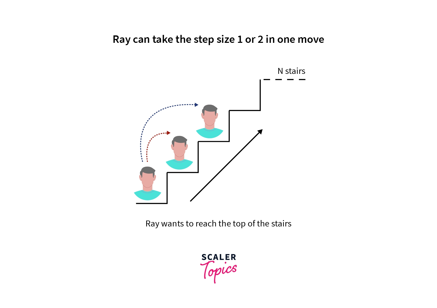
The problem Ray is facing is that he wants to count the number of ways he can reach the top of the stairs by taking the given type of steps.
For example, if we take a staircase of size 3 the total ways are counted as follows:
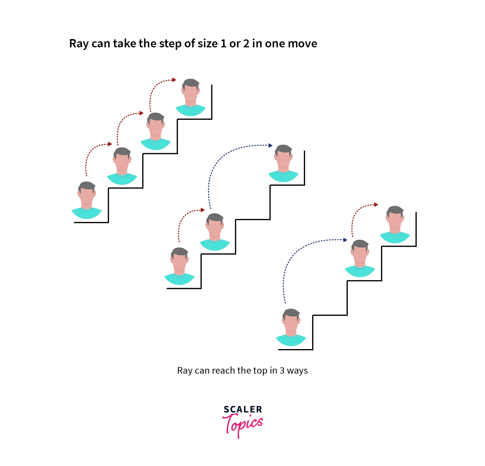
Hence, there are total 3 ways to reach the top, Now, for general case N how can we count the total number of ways.The solution lies in the fact that at each step one can move up in two ways either by 1 step or 2 step up and each of them contributes a unique way to final solution and we shall solve this by dynamic programming technique.
Let's see the formal definition of the above mentioned technique.
Dynamic programming is a very powerful programming technique used to solve a particular class of problems and it is based on a reccurence relationship which is further optimized in terms of time complexity at the cost of auxiliary space to solve the problem efficiently in terms of time complexity. Dynamic programming comes as an efficient programming technique which reduces the complexity of the problem to polynomial time complexity when techniques like brute-force, backtracking gives an exponential time time complexity for the same problems.
We shall learn to recognize the dynamic programming patterns in problems that occur in most of the programming contests and understand the underlying ideas of optimization and other observations.
Transform Your Career
Choose from our industry-leading programs designed for career success
Modern Software and AI Engineering Program
Master full-stack development with AI integration

Modern Data Science and ML with specialisation in AI
Advanced data science techniques with AI specialization
Advanced AIML with Specialisation in Agentic AI
Deep dive into AIML with focus on Agentic systems
DevOps, Cloud & AI Platform Engineering
Build and manage AI-powered cloud infrastructure
AI Engineering Advanced Certification by IIT-Roorkee
Premier AI engineering certification from IIT-Roorkee
General way to approach a dynamic programming (DP) problem
Highlights:
- A recurrence relation along with base cases is the key point to solve a dynamic programming problem.
- The staircase problem is yet another variation of famous fibbonaci series.
- Top-down approach starts from a larger input and goes down to the base case.
- Tabulation approach starts from base cases and builds the solution for the final input.
In this section, we shall learn to identify a dynamic programming problem and approach them with the appropriate techniques and work towards the best possible solution in terms of time and space complexity.
Let's take the same example of Ray trying to climb up the N stairs with jumps of length 1 and 2 and identify the dynamic programming patterns.
In this problem it can be seen that when Ray is at some Kth step (K > 2 and K <= N), then he must reach this step from K-1th step or K-2th step as shown
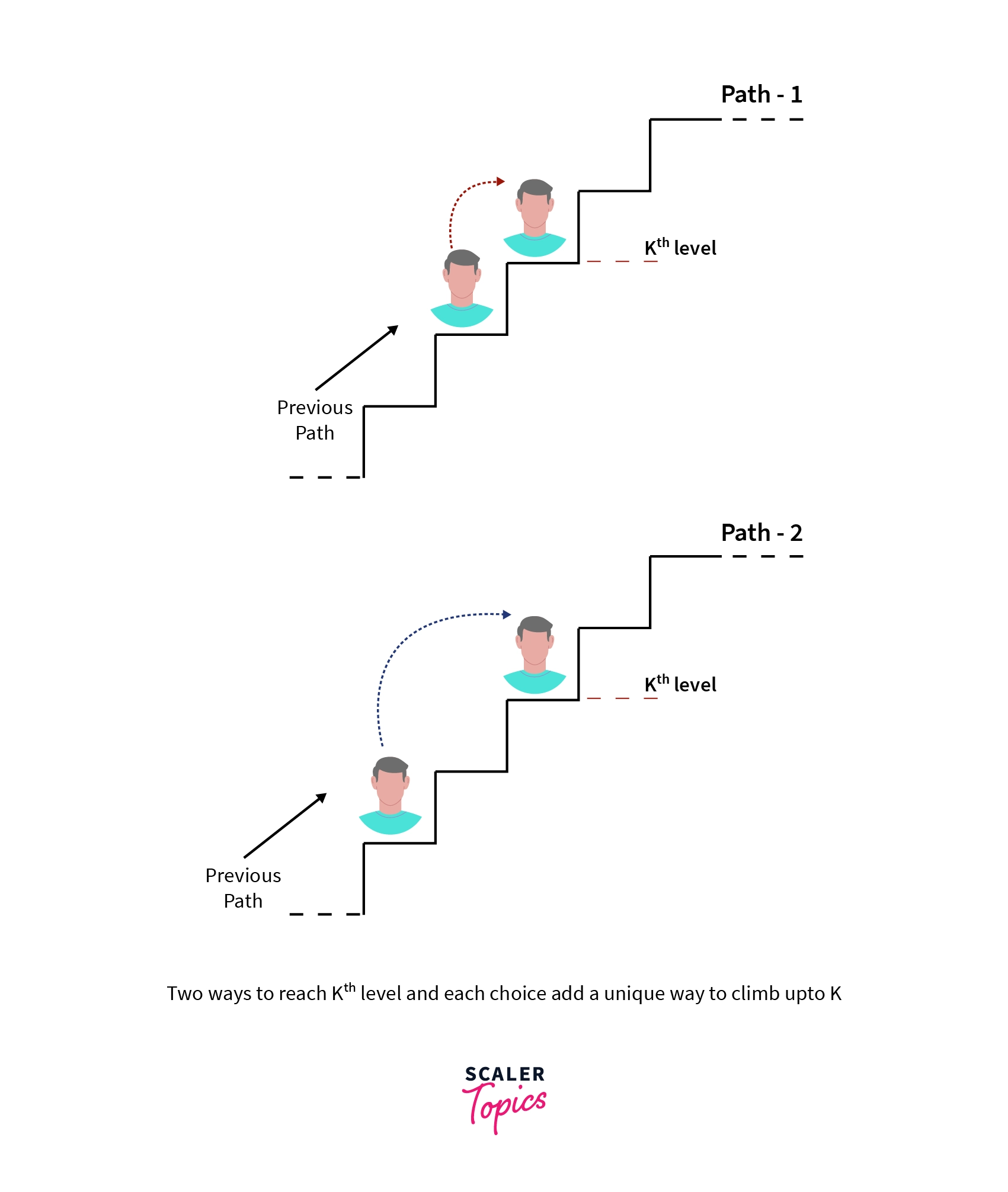
And each choice adds a unique path to the number of paths to reach K and this is true for all such K levels where K is in [1, N] inclusive.
Now, let's see how this observation can help us to build a solution.
Let's define a function f(k) which gives me the number of ways to reach the kth level ( k >= 1) and we know there are only two ways Ray can reach the kth level i.e. from k-1th and k-2th level, and the same function can be defined for these levels i.e. f(k-1) and f(k-2) and it becomes obvious that
In other words,
Number of ways to reach kth level = number of ways to reach k-1th level + number of ways to reach k-2th level
Now, k can be anything that makes the equation above holds and must be greater than or equal to 2.
The above-written equation is called a recurrence relation which we developed from the given information of the problem.
But when k < 2, then we have to make some changes to the equation and precompute these solutions beforehand and these cases are called base cases.
Hence, the base cases are k=1 , f(1) = 1 i.e. there is only one way to reach 1 that is to be at 1. k = 0, f(0) = 0 i.e. there are 0 ways to reach at step lesser than 1.
So, the final reccurence is as follows:
f(k) = f(k-1) + f(k-2), where k is the step number f(0) = 0 , f(1) = 1
The solution for some N say 4 can be visualized in terms of recursion tree as follows:
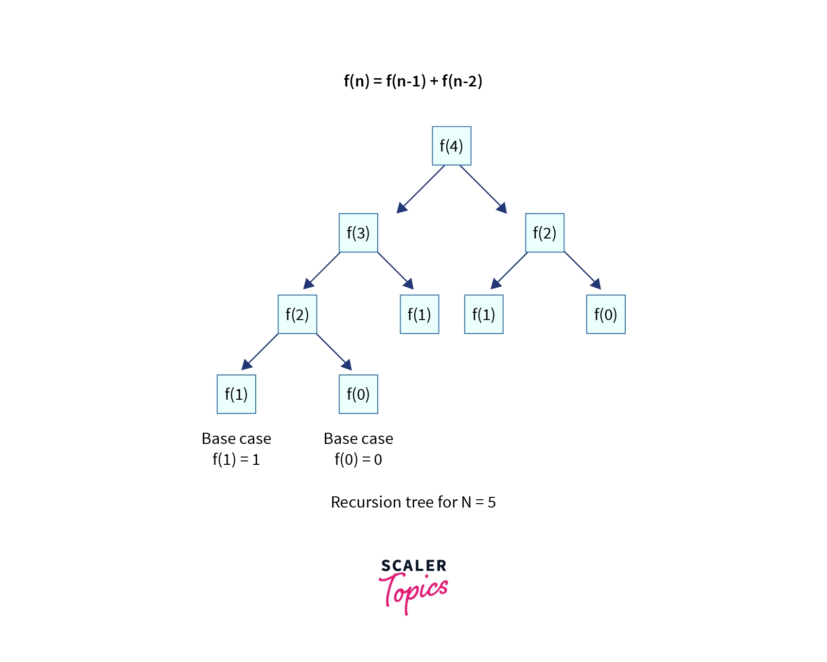
The above reccurence is familiar one, this is called fibbonaci series.
We have understood how to build a reccurence for a given problem and figure out the base cases for the same, now let's see the programming implementation of the recurrence.
The above reccurence can be implemented in C++ programming language as follows:
This is the recursive implementation of the count ways problem let's see the time and space requirements of the above program.
Time Complexity
We can observe that the recursion tree for an input of size N has exactly N levels and it forms a binary tree (each node has at most 2 children) and hence each level l has at most 2^l nodes which makes the worst-case time complexity to become which is exponential.
With this time complexity, even for a small input like , is more than iterations and we know that the time limit for the online judges is iterations per second and hence it will take seconds to execute the program for this very small input, Hence it is not a very good idea to use this approach for solving this problem.
Space Complexity:
This program does not take any auxiliary space but it uses a call stack hence, the space complexity is O(1).
Let's work towards the more optimal approach in terms of time complexity.
It can be noticed in the previous approach that for any N the recurrence keeps on reducing the input size N to make subproblems and keep solving those subproblems for these smaller input recursively until it reaches the base case for each such subproblem, in this process, many subproblems are repeated and solved again and again by the logic of the program as shown in the recurrence structure of the above Fibonacci series below:
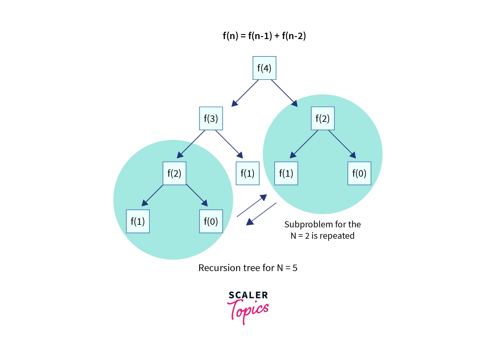
This type of property is called overlapping subproblems property and is one of the key properties of the dynamic programming problems.
To remove this extra computations one can simply store the results of each subproblem solved in some memo (or memory) such that when same problem is repeated its solution can be rendered in O(1).
But the above observation only helps when the solution of all subproblems is the most optimal solution for all of them then we can map that solution with the corresponding subproblem and the solution of the larger problem can be obtained using those solutions of subproblems this property is called optimal substructure property and the fibbonaci series satisfies both of these properties.
Hence, we use an array of size N to store the results of these computations such that when the same problem of some size k appears we can look into this array if we have the solution or not.
Let's see the working implementation in C++ programming language.
This type of optimization is called Memoization where we memoize the results of subproblems to be used later and this whole approach that we have explained till now is called the Top-down approach where we start from a larger input and keep breaking it down till the base case.
Let's understand the time and space complexity of the memoization appraoch:
Time Complexity: The key improvement of using a memo based solution is that the function is called for each node from 1 up to N exactly once and because after computing once the solution is already present in the table and can be retrieved in and the time complexity becomes .
Space Complexity: The space complexity becomes as we are using an extra array of size N, so we are improving time complexity at the cost of space complexity but the program will now work for larger inputs of size up to to be on safe side which is a huge improvement over the previous solution.
Let's understand a yet another way to approach the same problem and discuss its properties, time and space contraints.
In this approach we start from the base cases as indeed base cases are the optimal solutions of the smallest subproblems of the actual problem and here we see the optimal substructure property must hold i.e. we can always build the optimal solutions of larger subproblems from the optimal solutions of smaller subproblems.
Let's do the same for the above exampler problem, we start from base cases f(0) = 0, f(1) = 1 and we can compute the f(2) = f(0) + f(1), similarly f(3) and so on.
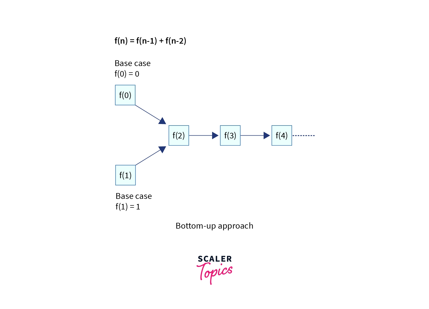
This approach is called Bottom-up appraoch.
Let's see the implementation of the above approach in C++ programming language:
The time and space complexity of the above approach is the same as the memoized solution.
With the above example, we learned two ways to tackle dynamic programming problems first is using Memoization (Top-down approach) and another is the Tabulation (Bottom-up approach).
The common thing in both of these approaches is the recurrence relation remains the same in both cases hence, before thinking of these approaches one needs to find the recurrence and then use further optimizations based on the given constraints of the problem.
In the next section we shall solve exampler problems related to dynamic programing in more than one dimensions of space although the idea discussed so far remains the same but can be generalized to any number of dimensions.
Exampler Problems
Highlights:
- Dynamic programming ideas can be generalized to any dimensions.
- Finding the minimum cost path in a cost matrix uses dynamic programming technique for optmizing solution.
- Minimum cost path can be backtracked using some stack data structure and backlinks.
- Find the number of ways to reach the bottom-right corner of a matrix.
- Find the number of ways to reach the bottom-right corner of a matrix with obstacles.
- Find the minimum number of operations required to convert string str1 to string str2.
In this section, we will extend the ideas explained previously into 2 dimensions and apply the same procedures to solve problems including dynamic programming patterns.
We shall discuss the standard problems of 2-dimensional dynamic programming techniques but the ideas remain the same and can be generalized to any problem in any number of dimensions.
1) Finding the Minimum Cost Path in a Grid when a Cost Matrix is given.
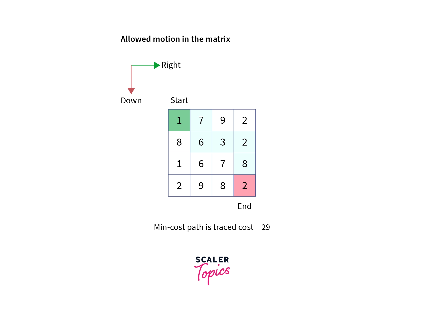
Given a cost matrix cost[][] of order N x M where cost[i][j] represents the cost of visiting the cell (i,j), find a minimum cost path to reach the bottom right cell (N-1,M-1) from cell (0,0) given that you can only travel one step right or one step down.
Note: we assume all costs are positive integers.
Example:
Let's work towards the solution of this problem.
We can see that the given motion is limited to only two directions i.e. right and down so to reach any position (i,j) in the matrix it must come from either the valid cell (i-1,j) or valid cell (i,j-1) for motion in downward direction and in right direction respectively.
First, to discuss the Top-down approach of the problem, we can start from the highest input value that is the ending cell in this case (N-1,M-1).
We can define a recursive function on the matrix say minCost(i,j) which gives the minimum cost path from cell (0,0) to (i,j). we start from the ending cell and Since we are allowed to move to right or down,for any cell (i,j) we need to choose between the minimum cost path between (0,0) to (i-1,j) and (0,0) to (i,j-1) and add the cost of the current cell (i,j). The corresponding reccurence is as follows:
Given that cells (i-1,j) and (i,j-1) are valid ones.
Base case: when (i,j) is (0,0) we return cost[0][0]
With the above recursive approach,time complexity of the programm becomes O(2^N) because at each cell we have exactly two options to move down and there are at most max(N,M) options encountered until base case is reached.
Let's work towards a bottom-up approach of the problem.
Given that we need to minimize the cost of the path so it is a minimization category of the dp problems and hence at each cell (i,j) we need to select the minimum cost path out of paths from (0,0) to (i-1,j) and (0,0) to (i,j-1) and once we select it we can extend it to add the current cell (i,j) by adding the cost[i][j] to the selected path.
To implement the above strategy we need to use an auxiliary matrix say minCost[][] of order NxM. where minCost[i][j] gives the minimum cost path from cell (0,0) to cell (i,j). The corresponding reccurence is
for all valid cells (i-1,j),(i,j-1),(i,j) such that 0 < i < N and 0 < j < M.
Base case: when (i,j) = (0,0) implies minCost[0][0] = cost[0][0].
After the computation is over, minCost[N-1][M-1] will contain the minimum cost path from (0,0) to (N-1,M-1). Let's see the implementation of the above solution in C++ programming language.
Let's discuss time and space complexity of the above approach:
Time Complexity:
Since we are building the minCost matrix and iterating over all cells it has O(NxM) time complexity which is far better than the recursive solution which gave exponential time complexity.
Space Complexity:
Since we are using extra space for the minCost matrix, the space complexity becomes O(NxM).
Again, we are improving time complexity at the cost of space.
Here, the follow-up question can be that one can ask to trace the exact path along with its cost. to do this back links can be used in another array and then the path is backtracked and stored in another path array or stack.
Let's see another variation of the same problem.
2) Finding the number of ways to reach from a starting position to an ending position travelling in specified directions only.
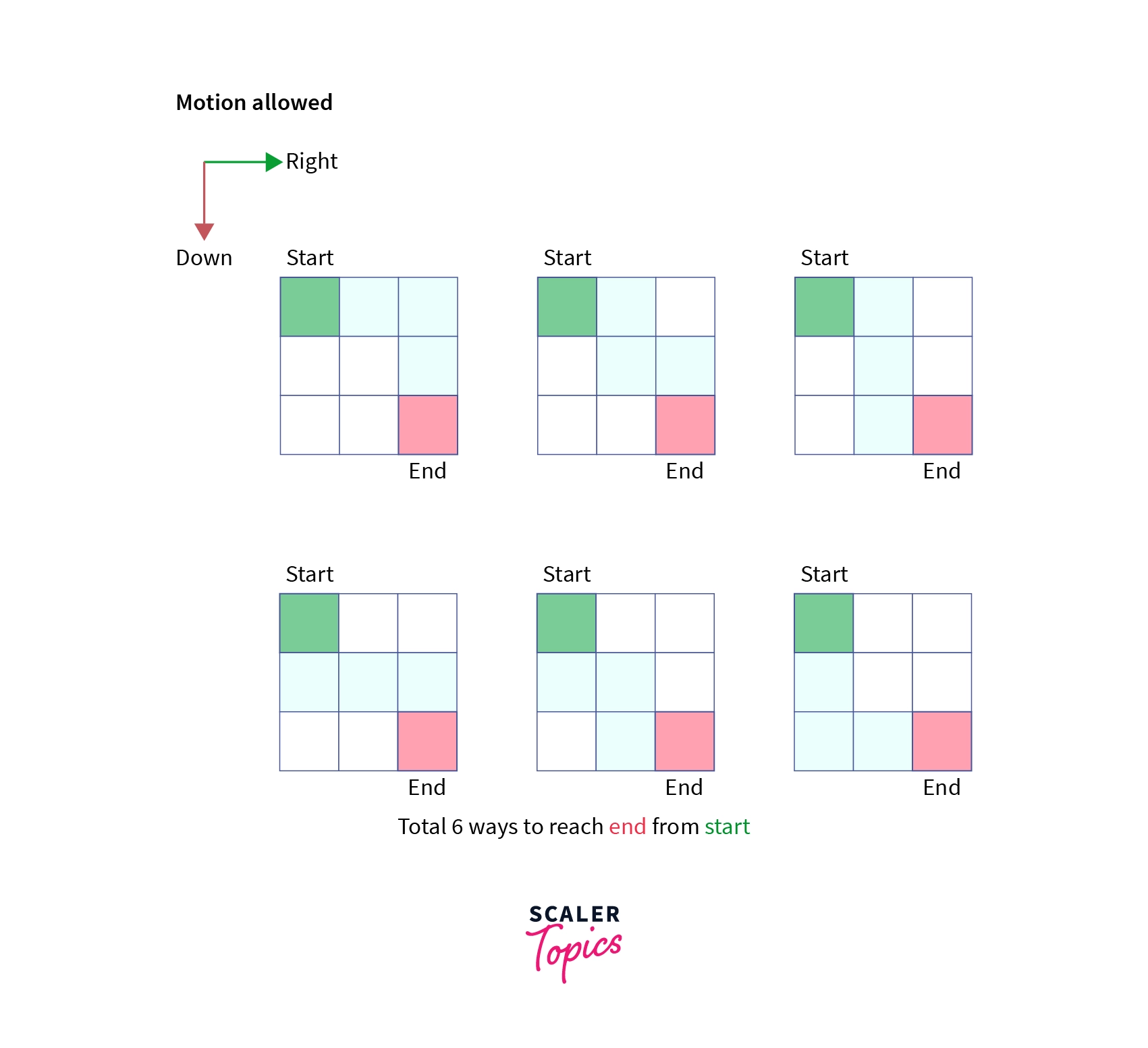
Given a 2-D matrix of order N x M, find the number of ways to reach cell with coordinates (i,j) from a starting cell (0,0), with the condition such that one can move only right and down one step.
Example: Suppose a matrix of order 3 x 3, the number of ways to reach the bottom right corner are shown below:
Let's work towards the solution of the above problem
Again, we can see that the motion is limited to the only right and downward direction and hence, to reach cell (i,j) one must come from valid (i-1,j) cell or (i,j-1) cell which accounts for the motion in downward and right direction respectively.
So, I can safely say that the number of ways to reach a cell (i,j) is equal to the sum of a number of ways to reach valid cell (i-1,j) and (i,j-1).
To start with Top-down approach, we define a recursive function countWays (i,j) which gives the number of ways to reach cell (i,j) starting from cell (0,0),we start from the ending cell (N-1,M-1) and recursively call the function countWays(i,j) for cells one step upward (i-1,j) and one step left (i,j-1) and add the resultant as follows.
such that 0 < i < N and 0 < j < M.
Base Case: cell (i,j) is starting cell (0,0) we return 1.
In base case, we return 1 because there is only one way to reach the starting cell that is to be at the starting point.
With the above recursive approach,time complexity of the program becomes O(2^N) because at each cell we have exactly two options to move down and there are at most max(N,M) options encountered until base case is reached.
Let's work towards a Bottom-up approach of the problem.
Given that we need to find the total ways to reach cell (i,j) starting from cell (0,0) and we can move either downward or right in one step, we just need to sum the number of ways to reach cell (i-1,j) from cell (0,0) and (i,j-1) from cell (0,0) because both sets can be extended to the current cell (i,j) by moving one step down and one step right.
To implement the above strategy, we need to declare an auxiliary matrix countWays[][] of order N x M where countWays[i][j] represents the number of ways to reach cell (i,j) starting from the cell (0,0).
The corresponding reccurence is as follows:
countWays[i][j] = countWays[i-1][j] + countWays[i][j-1] such that 0 < i < N and 0 < j < M
Base case: countWays[0][0] = 1, for cell (0,0).
Let's see the implementation of the same in C++ programming language.
Let's discuss the time and space complexity of the above implementation.
Time Complexity:
Since we are building the countWays matrix and iterating over all cells it has O(NxM) time complexity which is far better than the recursive solution which gave exponential time complexity.
Space complexity:
Since we are using extra space for the countWays matrix, the space complexity becomes O(NxM).
Again, we are improving time complexity at the cost of space.
3) Finding the number of ways to reach a particular position in a grid from a starting position (given some cells which are blocked).
Given a grid of order NxM and a robot on it which is designed to move on it, Robot is initially positioned at cell (0,0) i.e. the top-left cell, the Robot has to reach the end of the grid i.e. the cell (N-1, M-1). In a single step, Robot can move to its immediate right or immediate down provided the Robot is within the bounds on the grid and lands on a valid cell, there are some obstacles in the grid on random positions and the robot cannot land on those cells, your task is to compute the number of paths that the Robot can take to move from (1,1) to (N-1, M-1).
Example:
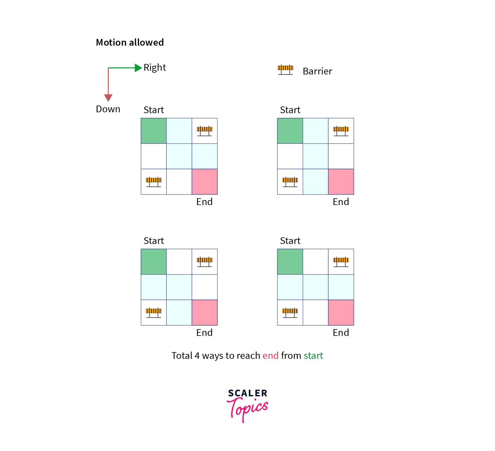
Let's work towards the solution of the above problem
Again, we can see that the motion is limited to the only right and downward direction and hence, to reach cell (i,j) one must come from valid (i-1,j) cell or (i,j-1) cell which accounts for the motion in downward and right direction respectively. But there are barriers in some cells and hence we need to handle some edge cases.
Case-1: In case the starting cell is blocked there is no way for the Robot to move in any direction and hence the answer is 0.
Case-2: In case the ending cell is blocked then there is no way for the Robot to reach that cell, hence the answer is 0.
Case-3: In cases where barriers occurs in cells other than starting and ending cells we can simply mark them with some unreasonable answer say -1 and simply skip that cell which contains -1.
Rest everything remains the same as in the previous solution.
Now, Let's see the implementation of the Bottom-up approach in C++ programming language:
Let's discuss the time and space complexity of the above implementation.
Time Complexity: Since we are building the countWays matrix and iterating over all cells it has O(NxM) time complexity which is far better than the recursive solution which gave exponential time complexity.
Space complexity: Since we are using extra space for the countWays matrix, the space complexity becomes O(NxM).
Again, we are improving time complexity at the cost of space.
Let's discuss one more problem of dynamic programming.
Scaler Placement Report and Statistics
Scaler learners achieved 2.5x salary growth with average post-Scaler CTC reaching ₹23L.
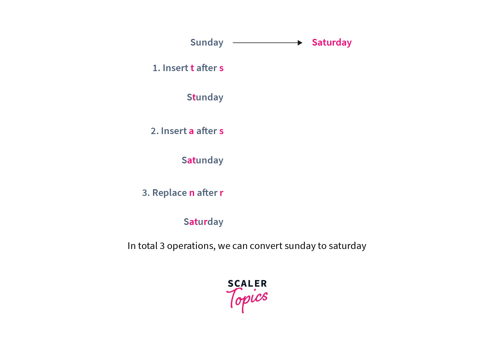
4) Edit Distance.
Given two strings str1 and str2 and a few operations that can be performed on str1, the task is to find the minimum number of operations required to convert str1 to str2. Operations:
- Insert.
- Delete.
- Replace.
Example:
Let's work towards the solution, we shall start with a recursive solution and then work towards the most optimized solution stepwise.
To find the recurrence, we need to find the subproblems and solve them recursively to get their solution, also we need a base case for this approach.
Assume the length of first string is N and of second is M and a recursive function editDistance(str1,str2,N,M) which gives the minimum edit distance to convert string str1 from index 0 to N-1 to str2 from index 0 to M-1, we start traversing both strings from ends and there can be two cases
currIndex1: pointer to the first string. currIndex2: pointer to the second string.
Initially, currIndex1 is N-1 and currIndex2 is M-1.
-
If the characters of both strings match then we simply skip this character and recur for the remaining strings i.e. for the string length currIndex1-1 and currIndex2-1 i.e. editDistance(str1,str2,currIndex1-1,currIndex2-1).
-
Else if the characters are not same then we need to consider all three operations on this character of the first string, we recursively calculate minimum cost for all three operations and take minimum of the three values obtained. a) Insert: we simply insert that character at currIndex1 position and move the currIndex2 to left i.e. recur for currIndex1 and currIndex2-1 i.e. editDistance(str1,str2,currIndex1,currIndex2-1).
b) Delete: we simply delete this mismatching character from the first string at currIndex1 position and move currIndex1 to left and try to match this character with the character at currIndex2 in second string i.e. recur for editDistance(str1,str2,currIndex1-1,currIndex2).
c) Replace: we simply replace the character at currIndex1 with the character at currIndex2 and move both pointers to the left i.e. recur for the editDistance(str1,str2,currIndex1-1,currIndex2-1).
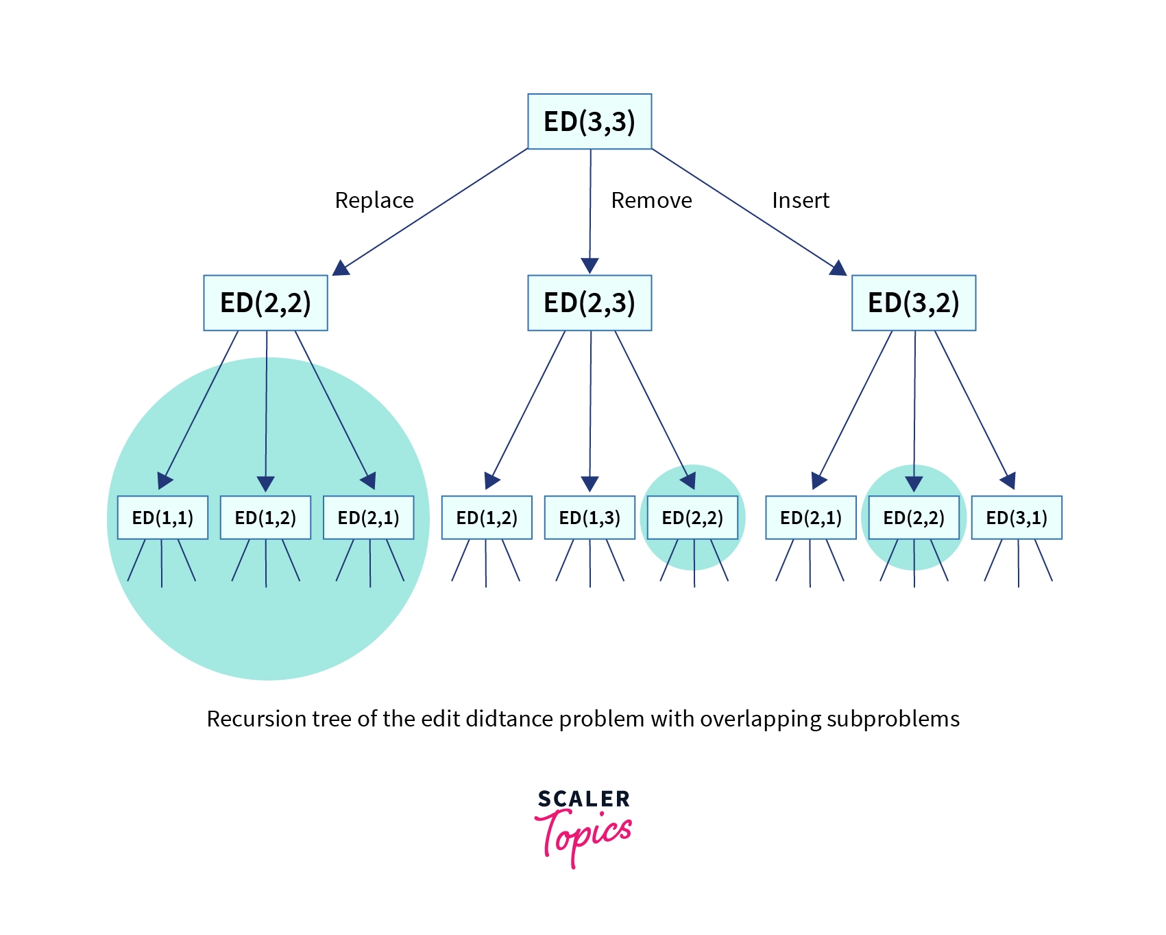
Same is depicted in the diagram below:
Let's see the implementation of the above strategy in C++ programming language:
Let's discuss the time and space complexity of the above program.
Time Complexity: There are exactly three function calls at each character in general and in the recursion tree we can see that it will have N levels and at each level l we have 3^l function calls and hence for N levels, we shall have 3^N function calls in the worst case, therefore, the worst-case time complexity is O(3^N) which is exponential.
Space complexity: Recursive solution does not consume any auxiliary space rather it makes use of call stack hence, O(1) space complexity.
This approach is not efficient for higher level inputs as explained before so we need to optimize this recursive solution and move towards a dynamic programming approach.
Given that there exists overlapping subproblems as shown in the image above, the problem has both properties of dynamic programming solution. let's build a bottom up approach for this problem.
We can define a dp as dp[i][j] represents the number of operations to convert string str1 of length i to str2 of length j.
The reccurence obviously remains the same but now we build the table in bottom up manner.
Base case: i == 0 , dp[i][j] = j
Base case: j == 0 , dp[i][j] = i
Let's see the C++ implementation of the above approach:
Let's discuss the time and space complexity of the above program.
Time complexity: We can see that we are using nested loops i.e. for each character of the first string str1, we are iterating over each character of second string str2 resulting in the time complexity of order O(NxM).
Space Complexity: We are using a dp table of order NxM, Hence space complexity is O(NxM).
:::
Conclusion
- We conclude that there are many type of problems that can be solved by dynamic programming technique.
- Some of them involves minimization ,maximization, counting the number of ways to accomplish some task.
- Occurence of keywords written in second point indicates the use of dynamic programming.
- Dynamic programming technique is generally an optimization of brutefore, backtracking/recursive solutions which gives exponential order of time complexity.
- Dynamic programming technique indeed improves the time complexity but at the cost of auxiliary space.