Relational Algebra in DBMS: Operators, Examples & SQL Equivalents
 FREE
FREE

Overview
Relational algebra is a procedural query language for relational databases. It takes one or more relations (tables) as input and produces a new relation as output, using a fixed set of operatorsselect, project, union, set difference, Cartesian product, and rename.
Every query you write in SQL is first compiled into a relational algebra expression by the database engine before execution. That translation step is exactly why relational algebra matters: understanding it gives you a window into how query optimizers work and why certain SQL patterns are faster than others.
Before reading this article, you should have some understanding of the following DBMS topics:
What is Relational Algebra in DBMS?
Relational Algebra came in 1970 and was given by Edgar F. Codd (Father of DBMS). It is also known as Procedural Query Language(PQL) as in PQL, a programmer/user has to mention two things, "What to Do" and "How to Do".
Suppose our data is stored in a database, then relational algebra is used to access the data from the database.
The First thing is we have to access the data, this needs to be specified in the query as "What to Do", but we have to also specify the method/procedure in the query that is "How to Do" or how to access the data from the database.
Stop learning AI in fragments—master a structured AI Engineering Course with hands-on GenAI systems with IIT Roorkee CEC Certification


AI Engineering Course Advanced Certification by IIT-Roorkee CEC
A hands on AI engineering program covering Machine Learning, Generative AI, and LLMs - designed for working professionals & delivered by IIT Roorkee in collaboration with Scaler.
Enrol Now
Types of Relational Operations in DBMS
In Relational Algebra, we have two types of Operations.
- Basic Operations
- Derived Operations
Applying these operations over relations/tables will give us new relations as output.

Basic Operations
Six fundamental operations are mentioned below. The majority of data retrieval operations are carried out by these. Let's know them one by one.
But, before moving into detail, let's have two tables or we can say relations STUDENT(ROLL, NAME, AGE) and EMPLOYEE(EMPLOYEE_NO, NAME, AGE) which will be used in the below examples.
STUDENT
| ROLL | NAME | AGE |
|---|---|---|
| 1 | Aman | 20 |
| 2 | Atul | 18 |
| 3 | Baljeet | 19 |
| 4 | Harsh | 20 |
| 5 | Prateek | 21 |
| 6 | Prateek | 23 |
EMPLOYEE
| EMPLOYEE_NO | NAME | AGE |
|---|---|---|
| E-1 | Anant | 20 |
| E-2 | Ashish | 23 |
| E-3 | Baljeet | 25 |
| E-4 | Harsh | 20 |
| E-5 | Pranav | 22 |
Select (σ)
Select operation is done by Selection Operator which is represented by "sigma"(σ). It is used to retrieve tuples(rows) from the table where the given condition is satisfied. It is a unary operator means it requires only one operand.
Notation : σ p(R)
Where σ is used to represent SELECTION
R is used to represent RELATION
p is the logic formula
Let's understand this with an example:
Suppose we want the row(s) from STUDENT Relation where "AGE" is 20
This will return the following output:
| ROLL | NAME | AGE |
|---|---|---|
| 1 | Aman | 20 |
| 4 | Harsh | 20 |
Build an AI-First Career, Master the Complete Skillset
Choose from our industry-leading programs designed for career success
Modern Software and AI Engineering Program
Master full-stack development with AI integration


 +1000 more
Modern Data Science and ML with specialisation in AI
Advanced data science techniques with AI specialization
+1000 moreAdvanced AIML with Specialisation in Agentic AI
Deep dive into AIML with focus on Agentic systems
+1000 moreDevOps, Cloud & AI Platform Engineering
Build and manage AI-powered cloud infrastructure
+1000 moreAI Engineering Advanced Certification by IIT-Roorkee
Premier AI engineering certification from IIT-Roorkee

AI Forward Deployed Engineer Program
Full-stack engineering, production AI and client-facing consulting
+1000 moreProject (∏)
Project operation is done by Projection Operator which is represented by "pi"(∏). It is used to retrieve certain attributes(columns) from the table. It is also known as vertical partitioning as it separates the table vertically. It is also a unary operator.
Notation : ∏ a(r)
Where ∏ is used to represent PROJECTION
r is used to represent RELATION
a is the attribute list
Let's understand this with an example:
Suppose we want the names of all students from STUDENT Relation.
This will return the following output:
| NAME |
|---|
| Aman |
| Atul |
| Baljeet |
| Harsh |
| Prateek |
As you can see from the above output it eliminates duplicates.
For multiple attributes, we can separate them using a ",".
Above code will return two columns, ROLL and NAME.
| ROLL | NAME |
|---|---|
| 1 | Aman |
| 2 | Atul |
| 3 | Baljeet |
| 4 | Harsh |
| 5 | Prateek |
| 6 | Prateek |
Union (∪)
Union operation is done by Union Operator which is represented by "union"(∪). It is the same as the union operator from set theory, i.e., it selects all tuples from both relations but with the exception that for the union of two relations/tables both relations must have the same set of Attributes. It is a binary operator as it requires two operands.
Notation: R ∪ S
Where R is the first relation
S is the second relation
If relations don't have the same set of attributes, then the union of such relations will result in NULL.
Let's have an example to clarify the concept:
Suppose we want all the names from STUDENT and EMPLOYEE relation.
| NAME |
|---|
| Aman |
| Anant |
| Ashish |
| Atul |
| Baljeet |
| Harsh |
| Pranav |
| Prateek |
As we can see from the above output it also eliminates duplicates.
Set Difference (-)
Set Difference as its name indicates is the difference between two relations (R-S). It is denoted by a "Hyphen"(-) and it returns all the tuples(rows) which are in relation R but not in relation S. It is also a binary operator.
Notation : R - S
Where R is the first relation
S is the second relation
Just like union, the set difference also comes with the exception of the same set of attributes in both relations.
Let's take an example where we would like to know the names of students who are in STUDENT Relation but not in EMPLOYEE Relation.
This will give us the following output:
| NAME |
|---|
| Aman |
| Atul |
| Prateek |
Cartesian product (X)
Cartesian product is denoted by the "X" symbol. Let's say we have two relations R and S. Cartesian product will combine every tuple(row) from R with all the tuples from S. I know it sounds complicated, but once we look at an example, you'll see what I mean.
Notation: R X S
Where R is the first relation
S is the second relation
As we can see from the notation it is also a binary operator.
Let's combine the two relations STUDENT and EMPLOYEE.
| ROLL | NAME | AGE | EMPLOYEE_NO | NAME | AGE |
|---|---|---|---|---|---|
| 1 | Aman | 20 | E-1 | Anant | 20 |
| 1 | Aman | 20 | E-2 | Ashish | 23 |
| 1 | Aman | 20 | E-3 | Baljeet | 25 |
| 1 | Aman | 20 | E-4 | Harsh | 20 |
| 1 | Aman | 20 | E-5 | Pranav | 22 |
| 2 | Atul | 18 | E-1 | Anant | 20 |
| 2 | Atul | 18 | E-2 | Ashish | 23 |
| 2 | Atul | 18 | E-3 | Baljeet | 25 |
| 2 | Atul | 18 | E-4 | Harsh | 20 |
| 2 | Atul | 18 | E-5 | Pranav | 22 |
. . . And so on.
Rename (ρ)
Rename operation is denoted by "Rho"(ρ). As its name suggests it is used to rename the output relation. Rename operator too is a binary operator.
Notation: ρ(R,S)
Where R is the new relation name
S is the old relation name
Let's have an example to clarify this
Suppose we are fetching the names of students from STUDENT relation. We would like to rename this relation as STUDENT_NAME.
STUDENT_NAME
| NAME |
|---|
| Aman |
| Atul |
| Baljeet |
| Harsh |
| Prateek |
As you can see, this output relation is named "STUDENT_NAME".
Takeaway
- Select (σ) is used to retrieve tuples(rows) based on certain conditions.
- Project (∏) is used to retrieve attributes(columns) from the relation.
- Union (∪) is used to retrieve all the tuples from two relations.
- Set Difference (-) is used to retrieve the tuples which are present in R but not in S(R-S).
- Cartesian product (X) is used to combine each tuple from the first relation with each tuple from the second relation.
- Rename (ρ) is used to rename the output relation.
Master structured AI Engineering + GenAI hands-on, earn IIT Roorkee CEC Certification at ₹40,000
AI Engineering Course Advanced Certification by IIT-Roorkee CEC
A hands on AI engineering program covering Machine Learning, Generative AI, and LLMs - designed for working professionals & delivered by IIT Roorkee in collaboration with Scaler.
Enrol NowDerived Operations
Also known as extended operations, these operations can be derived from basic operations and hence named Derived Operations. These include three operations: Join Operations, Intersection operations, and Division operations.
Let's study them one by one.
Join Operations
Join Operation in DBMS are binary operations that allow us to combine two or more relations.
They are further classified into two types: Inner Join, and Outer Join.
First, let's have two relations EMPLOYEE consisting of E_NO, E_NAME, CITY and EXPERIENCE. EMPLOYEE table contains employee's information such as id, name, city, and experience of employee(In Years). The other relation is DEPARTMENT consisting of D_NO, D_NAME, E_NO and MIN_EXPERIENCE.
DEPARTMENT table defines the mapping of an employee to their department. It contains Department Number, Department Name, Employee Id of the employee working in that department, and the minimum experience required(In Years) to be in that department.
EMPLOYEE
| E_NO | E_NAME | CITY | EXPERIENCE |
|---|---|---|---|
| E-1 | Ram | Delhi | 04 |
| E-2 | Varun | Chandigarh | 09 |
| E-3 | Ravi | Noida | 03 |
| E-4 | Amit | Bangalore | 07 |
DEPARTMENT
| D_NO | D_NAME | E_NO | MIN_EXPERIENCE |
|---|---|---|---|
| D-1 | HR | E-1 | 03 |
| D-2 | IT | E-2 | 05 |
| D-3 | Marketing | E-3 | 02 |
Also, let's have the Cartesian Product of the above two relations. It will be much easier to understand Join Operations when we have the Cartesian Product.
| E_NO | E_NAME | CITY | EXPERIENCE | D_NO | D_NAME | E_NO | MIN_EXPERIENCE |
|---|---|---|---|---|---|---|---|
| E-1 | Ram | Delhi | 04 | D-1 | HR | E-1 | 03 |
| E-1 | Ram | Delhi | 04 | D-2 | IT | E-2 | 05 |
| E-1 | Ram | Delhi | 04 | D-3 | Marketing | E-3 | 02 |
| E-2 | Varun | Chandigarh | 09 | D-1 | HR | E-1 | 03 |
| E-2 | Varun | Chandigarh | 09 | D-2 | IT | E-2 | 05 |
| E-2 | Varun | Chandigarh | 09 | D-3 | Marketing | E-3 | 02 |
| E-3 | Ravi | Noida | 03 | D-1 | HR | E-1 | 03 |
| E-3 | Ravi | Noida | 03 | D-2 | IT | E-2 | 05 |
| E-3 | Ravi | Noida | 03 | D-3 | Marketing | E-3 | 02 |
| E-4 | Amit | Bangalore | 07 | D-1 | HR | E-1 | 03 |
| E-4 | Amit | Bangalore | 07 | D-2 | IT | E-2 | 05 |
| E-4 | Amit | Bangalore | 07 | D-3 | Marketing | E-3 | 02 |
Inner Join
When we perform Inner Join, only those tuples returned that satisfy the certain condition. It is also classified into three types: Theta Join, Equi Join and Natural Join.
Theta Join (θ)
Theta Join combines two relations using a condition. This condition is represented by the symbol "theta"(θ). Here conditions can be inequality conditions such as >,<,>=,<=, etc.
Notation : R ⋈θ S
Where R is the first relation
S is the second relation
Let's have a simple example to understand this.
Suppose we want a relation where EXPERIENCE from EMPLOYEE >= MIN_EXPERIENCE from DEPARTMENT.
| E_NO | E_NAME | CITY | EXPERIENCE | D_NO | D_NAME | E_NO | MIN_EXPERIENCE |
|---|---|---|---|---|---|---|---|
| E-1 | Ram | Delhi | 04 | D-1 | HR | E-1 | 03 |
| E-1 | Ram | Delhi | 04 | D-3 | Marketing | E-3 | 02 |
| E-2 | Varun | Chandigarh | 09 | D-1 | HR | E-1 | 03 |
| E-2 | Varun | Chandigarh | 09 | D-2 | IT | E-2 | 05 |
| E-2 | Varun | Chandigarh | 09 | D-3 | Marketing | E-3 | 02 |
| E-3 | Ravi | Noida | 03 | D-1 | HR | E-1 | 03 |
| E-3 | Ravi | Noida | 03 | D-3 | Marketing | E-3 | 02 |
| E-4 | Amit | Bangalore | 07 | D-1 | HR | E-1 | 03 |
| E-4 | Amit | Bangalore | 07 | D-2 | IT | E-2 | 05 |
| E-4 | Amit | Bangalore | 07 | D-3 | Marketing | E-3 | 02 |
Check the Cartesian Product, if in any tuple/row EXPERIENCE >= MIN_EXPERIENCE then insert this tuple/row in output relation.
Equi Join
Equi Join is a special case of theta join where the condition can only contain **equality(=)** comparisons.
A non-equijoin is the inverse of an equi join, which occurs when you join on a condition other than "=".
Let's have an example where we would like to join EMPLOYEE and DEPARTMENT relation where E_NO from EMPLOYEE = E_NO from DEPARTMENT.
| E_NO | E_NAME | CITY | EXPERIENCE | D_NO | D_NAME | E_NO | MIN_EXPERIENCE |
|---|---|---|---|---|---|---|---|
| E-1 | Ram | Delhi | 04 | D-1 | HR | E-1 | 03 |
| E-2 | Varun | Chandigarh | 09 | D-2 | IT | E-2 | 05 |
| E-3 | Ravi | Noida | 03 | D-3 | Marketing | E-3 | 02 |
Check Cartesian Product, if the tuple contains same E_NO, insert that tuple in the output relation
Natural Join (⋈)
A comparison operator is not used in a natural join. It does not concatenate like a Cartesian product. A Natural Join can be performed only if two relations share at least one common attribute. Furthermore, the attributes must share the same name and domain.
Natural join operates on matching attributes where the values of the attributes in both relations are the same and remove the duplicate ones.
Preferably Natural Join is performed on the foreign key.
Notation : R ⋈ S
Where R is the first relation
S is the second relation
Let's say we want to join EMPLOYEE and DEPARTMENT relation with E_NO as a common attribute.
Notice, here E_NO has the same name in both the relations and also consists of the same domain, i.e., in both relations E_NO is a string.
| E_NO | E_NAME | CITY | EXPERIENCE | D_NO | D_NAME | MIN_EXPERIENCE |
|---|---|---|---|---|---|---|
| E-1 | Ram | Delhi | 04 | D-1 | HR | 03 |
| E-2 | Varun | Chandigarh | 09 | D-2 | IT | 05 |
| E-3 | Ravi | Noida | 03 | D-3 | Marketing | 02 |
But unlike the above operation, where we have two columns of E_NO, here we are having only one column of E_NO. This is because Natural Join automatically keeps a single copy of a common attribute.
How Scaler Transformed Careers in Different Fields
Scaler learners achieved 2.5x salary growth with average post-Scaler CTC reaching ₹23L.
 Google
 Amazon
 Microsoft
 Flipkart
 Adobe1200+ more
Become the Ai engineer who can design, build, and iterate real AI products, not just demos with an IIT Roorkee CEC Certification
AI Engineering Course Advanced Certification by IIT-Roorkee CEC
A hands on AI engineering program covering Machine Learning, Generative AI, and LLMs - designed for working professionals & delivered by IIT Roorkee in collaboration with Scaler.
Enrol NowOuter Join
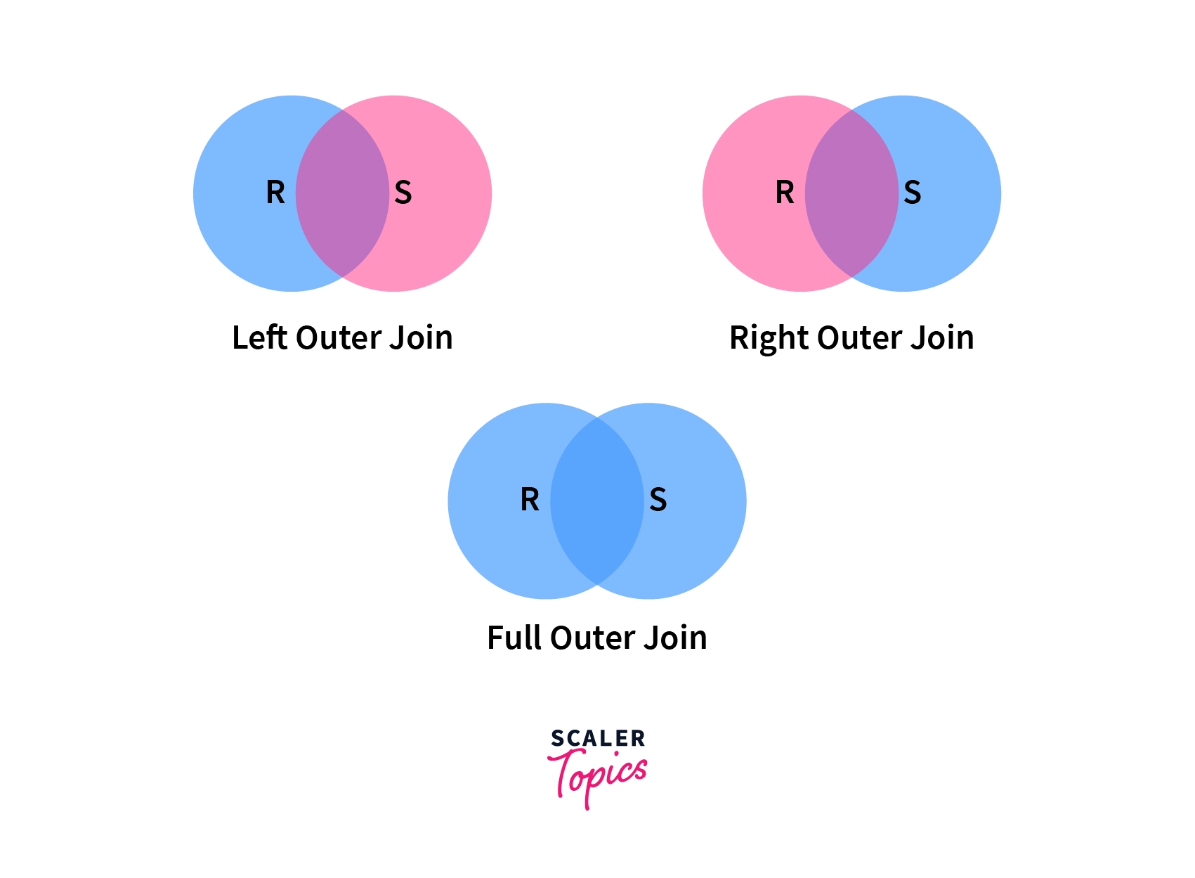
Unlike Inner Join which includes the tuple that satisfies the given condition, Outer Join also includes some/all the tuples which don't satisfy the given condition. It is also of three types: Left Outer Join, Right Outer Join, and Full Outer Join.
Let's say we have two relations R and S, then
Below is the representation of Left, Right, and Full Outer Joins.
Left Outer Join
As we can see from the diagram, Left Outer Join returns the matching tuples(tuples present in both relations) and the tuples which are only present in Left Relation, here R.
However, if the matching tuples are NULL, then attributes/columns of Right Relation, here S are made NULL in the output relation.
Let's understand this a bit more using an example:
Here we are combining EMPLOYEE and DEPARTMENT relation with the constraint that EMPLOYEE's E_NO must be equal to DEPARTMENT's E_NO.
| E_NO | E_NAME | CITY | EXPERIENCE | D_NO | D_NAME | MIN_EXPERIENCE |
|---|---|---|---|---|---|---|
| E-1 | Ram | Delhi | 04 | D-1 | HR | 03 |
| E-2 | Varun | Chandigarh | 09 | D-2 | IT | 05 |
| E-3 | Ravi | Noida | 03 | D-3 | Marketing | 02 |
| E-4 | Amit | Bangalore | 07 | - | - | - |
As you can see here, all the tuples from left, i.e., EMPLOYEE relation are present. But E-4 is not satisfying the given condition, i.e., E_NO from EMPLOYEE must be equal to E_NO from DEPARTMENT, still it is included in the output relation. This is because Outer Join also includes some/all the tuples which don't satisfy the condition. That's why Outer Join marked E-4's corresponding tuple/row from DEPARTMENT as NULL.
Right Outer Join
Right Outer Join returns the matching tuples and the tuples which are only present in Right Relation here S.
The same happens with the Right Outer Join, if the matching tuples are NULL, then the attributes of Left Relation, here R are made NULL in the output relation.
We will combine EMPLOYEE and DEPARTMENT relations with the same constraint as above.
| E_NO | E_NAME | CITY | EXPERIENCE | D_NO | D_NAME | MIN_EXPERIENCE |
|---|---|---|---|---|---|---|
| E-1 | Ram | Delhi | 04 | D-1 | HR | 03 |
| E-2 | Varun | Chandigarh | 09 | D-2 | IT | 05 |
| E-3 | Ravi | Noida | 03 | D-3 | Marketing | 02 |
As all the tuples from DEPARTMENT relation have a corresponding E_NO in EMPLOYEE relation, therefore no tuple from EMPLOYEE relation contains a NULL.
Full Outer Join
Full Outer Join returns all the tuples from both relations. However, if there are no matching tuples then, their respective attributes are made NULL in output relation.
Again, combine the EMPLOYEE and DEPARTMENT relation with the same constraint.
| E_NO | E_NAME | CITY | EXPERIENCE | D_NO | D_NAME | MIN_EXPERIENCE |
|---|---|---|---|---|---|---|
| E-1 | Ram | Delhi | 04 | D-1 | HR | 03 |
| E-2 | Varun | Chandigarh | 09 | D-2 | IT | 05 |
| E-3 | Ravi | Noida | 03 | D-3 | Marketing | 02 |
| E-4 | Amit | Bangalore | 07 | - | - | - |
Intersection (∩)
Intersection operation is done by Intersection Operator which is represented by "intersection"(∩).It is the same as the intersection operator from set theory, i.e., it selects all the tuples which are present in both relations. It is a binary operator as it requires two operands. Also, it eliminates duplicates.
Notation : R ∩ S
Where R is the first relation
S is the second relation
Let's have an example to clarify the concept:
Suppose we want the names which are present in STUDENT as well as in EMPLOYEE relation, Relations we used in Basic Operations.
| NAME |
|---|
| Baljeet |
| Harsh |
Division (÷)
Division Operation is represented by "division"(÷ or /) operator and is used in queries that involve keywords "every", "all", etc.
Notation : R(X,Y)/S(Y)
Here,
R is the first relation from which data is retrieved.
S is the second relation that will help to retrieve the data.
X and Y are the attributes/columns present in relation. We can have multiple attributes in relation, but keep in mind that attributes of S must be a proper subset of attributes of R.
For each corresponding value of Y, the above notation will return us the value of X from tuple<X,Y> which exists everywhere.
It's a bit difficult to understand this in a theoretical way, but you will understand this with an example.
Let's have two relations, ENROLLED and COURSE. ENROLLED consist of two attributes STUDENT_ID and COURSE_ID. It denotes the map of students who are enrolled in given courses.
COURSE contains the list of courses available.
See, here attributes/columns of COURSE relation are a proper subset of attributes/columns of ENROLLED relation. Hence Division operation can be used here.
ENROLLED
| STUDENT_ID | COURSE_ID |
|---|---|
| Student_1 | DBMS |
| Student_2 | DBMS |
| Student_1 | OS |
| Student_3 | OS |
COURSE
| COURSE_ID |
|---|
| DBMS |
| OS |
Now the query is to return the STUDENT_ID of students who are enrolled in every course.
This will return the following relation as output.
| STUDENT_ID |
|---|
| Student_1 |
Turn Learning into Career Growth
Takeaway
- Theta Join (θ) combines two relations based on a condition.
- Equi Join is a type of Theta Join where only equality condition (=) is used.
- Natural Join (⋈) combines two relations based on a common attribute (preferably foreign key).
- Left Outer Join (⟕) returns the matching tuples and tuples which are only present in the left relation.
- Right Outer Join (⟖) returns the matching tuples and tuples which are only present in the right relation.
- Full Outer Join (⟗) returns all the tuples present in the left and right relations.
FAQs
What is relational algebra in DBMS?
Relational algebra is a procedural query language that takes one or two relations as input and produces a new relation as output, using operators such as select (σ), project (π), union (∪), set difference (−), Cartesian product (×) and rename (ρ). It forms the theoretical foundation of SQL and is the internal language that database query optimizers use to plan execution strategies.
What are the 5 basic operations of relational algebra?
The five basic operations of relational algebra are Select (σ), Project (π), Union (∪), Set Difference (−), and Cartesian Product (×). Rename (ρ) is often counted as a sixth fundamental operator. Every other operation join, intersection, division, outer joins—can be derived from these six.
What is the relational algebra?
It is the formal, procedural language of the relational model: relations go in, a relation comes out. It matters because it is the language a query optimizer reasons in every SQL query is translated into a relational algebra tree before the database executes it, and the optimizer can rearrange that tree to improve performance without changing the result. Source: Silberschatz, Korth & Sudarshan, Database System Concepts, 7th Edition
What is an example of a relational DBMS?
MySQL, PostgreSQL, Oracle Database, Microsoft SQL Server and SQLite are relational database management systems. They store data as relations (tables) and expose a query language grounded in relational algebra. Each of these systems compiles SQL into an internal algebra representation for optimization.
Is relational algebra procedural or non-procedural?
Procedural. It specifies how to compute the result as an ordered sequence of operations you write σ first, then π, then ⋈. Relational calculus is the non-procedural counterpart, specifying only what the result should contain and leaving the execution order to the database engine.
What is the difference between natural join and equi join?
An equi join joins on an equality condition and keeps both joining columns in the result. A natural join joins automatically on all common attributes and keeps the common column once. Every natural join is an equi join with duplicate columns removed—but natural join's automatic column selection can silently join on the wrong attribute if two columns share a name unintentionally. Source: MySQL Documentation JOIN
What is the division operator used for?
For "for all" queries finding tuples related to every value in another relation, such as students enrolled in every course. SQL has no division operator; it is emulated with GROUP BY ... HAVING COUNT(DISTINCT ...) = (SELECT COUNT(*) FROM divisor) or a double NOT EXISTS subquery. In our worked example, only Aarav (roll_no 101) was enrolled in all three courses.
Is relational algebra important for GATE and semester exams?
Yes. Expression-writing questions, operator equivalence, and division-operator problems appear regularly in GATE, UGC NET, and university DBMS examinations. The algebra–calculus equivalence (Codd's theorem) is a standard theory question, and join-type distinctions (natural vs equi vs theta vs outer) are perennial exam favourites. The self-join pattern for finding the maximum without aggregates (Problem 5) is a GATE classic.
Conclusion
Relational algebra is the procedural backbone of the relational model six basic operators (σ, π, ρ, ∪, −, ×) from which everything else is derived. Join, intersection, and division are shorthand for expressions built from these six. Every SQL query is compiled into a relational algebra tree by the database engine, and the optimizer uses that tree to find the fastest execution plan, which is why writing SQL declaratively does not mean the database computes naively.
Relational calculus is the declarative twin: Codd proved the two are equivalent in expressive power (relational completeness), meaning any query expressible in one is expressible in the other. The calculus specifies what you want; the algebra specifies how to get it. Modern SQL sits closer to the calculus in spirit but compiles to the algebra in practice.
For any DBMS exam GATE, semester test, or placement interview the essentials are: write expressions in the right order (select before project), remember that natural join silently drops dangling tuples (hence outer joins), know that division answers "for all" questions, and remember that rename is the operator that makes self-joins possible. Master these, and every relational algebra question becomes a pattern match.
Sources and References:
- Codd, E.F., "A Relational Model of Data for Large Shared Data Banks," Communications of the ACM, Vol. 13, No. 6, June 1970. DOI
- Silberschatz, Korth & Sudarshan, Database System Concepts, 7th Edition. db-book.com
- Elmasri & Navathe, Fundamentals of Database Systems, 7th Edition
- ISO/IEC 9075 — Information Technology — Database Languages — SQL. iso.org
- PostgreSQL Documentation: JOIN Syntax. postgresql.org
- MySQL 8.0 Reference Manual: JOIN. dev.mysql.com
Reviewed by: Scaler Curriculum Team
Tags: DBMS, Relational Algebra, SQL, Database Management, Query Language, Operators, Relational Calculus, GATE, Interview Prep
Conclusion
- Relational Algebra in DBMS is a theoretical model which is the fundamental block for SQL. It comprises different mathematics operations.
- Operations are divided into two main categories: Basic and Derived.
- Basic consists of six Operations: SELECT, PROJECT, UNION, SET DIFFERENCE, CARTESIAN PRODUCT, RENAME.
- Derived Consist of three Operations: JOINS, INTERSECTION, DIVISION.
- Joins are of two types: Inner Join and Outer Join . Inner Join is further classified into three types: Theta Join, Equi Join, and Natural Join. Outer Join also consists of three types: Left Outer Join, Right Outer Join, and Full Outer Join.