Stable Sorting Algorithm

Different Types Of Sorting Algorithms

Sorting is one of the most thoroughly studied algorithms in computer science. There are different sorting implementations and applications that we can use to make our code more efficient and effective.

Let us study them one by one.

Bubble Sort

• Bubble sort is one of the simplest and most straightforward sorting algorithms that work by comparing elements in a list, which are adjacent (next to each other) and then swapping them, until the largest(or smallest) of them reaches its correct order.
• In real life, bubble sort can be visualized when people in a queue waiting to be standing in a height-wise sorted manner swap their positions among themselves until everyone is standing based on the increasing order of heights.

How does bubble sort work?

Consider that we want to sort a list in ascending order. To perform this sorting, the bubble sort algorithm will follow the below steps :

1. Begin with the first element.
2. Compare the current element with the next element.
3. If the current element is greater than the next element, then swap both the elements. If not, move to the next element.
4. Repeat steps 1 – 3 until we get the sorted list.

To better understand bubble sort, let us take the example of a list containing $4$ elements. The steps to sort this list would involve :

From the above-given diagram, we can infer or conclude the following conclusions about the bubble sort algorithm :

• In bubble sort, to sort a list of length n, we need to perform n – 1 iterations. For example, we had 4 elements in our list, and we got them sorted in 3 passes. After our 3rd pass, we got a sorted list. While we reach the (n – 1)th iteration, we are only left with one element. And, since the 1 element is already sorted, we don't need to perform any more comparisons.
• Second observation is, in the first pass, the highest element (9 in this case) was bubbled out on the right-most side of the list. Similarly, after each iteration, the largest among the unsorted elements was placed at its position. Hence, this sorting algorithm is known as bubble sort.
• In the second pass, we did not compare elements 7 and 8. Because, we know that 8 is already at its correct position, and comparing them would not make any difference. So, in each pass, comparison occurs up to the last unsorted element. Through this, we can reduce the number of comparisons.

Bubble sort algorithm

We just saw that to sort a list of n elements using bubble sort, we need to perform n – 1 iteration. And for each iteration, we need to :

• Run a loop over the entire list or array.
• Compare the element at the index $i$ with the element at $(i + 1)$.
• If the element at $i$ is greater than the element at $(i + 1)$, swap both the elements
• Else, move to the next element.

Pseudocode :

Time complexity analysis

Let us analyze the time complexity of bubble sort through the following steps:

In bubble sort, we have:

1. One loop(outer loop) to iterate over the entire list
2. Another loop(inner loop) to iterate over the list to compare the adjacent elements.

Let the number of elements in the list be $n$. Now, we know that for part 1, the loop would run for n times. And, each iteration of the loop would take constant time. Hence, for the first loop, the time complexity would be $O(n)$.

Now, in part 2, our other loop is nested inside the loop that is run in part 1. In this part, n comparisons are made, that take constant time for execution. In simple words, each time our part 1's loop(outer loop) is executed, the part 2 loop (inner loop) will execute $n$ times.

So, if part 1 is executed for $n$ number of times, part 2 would be executed for $n * n$ number of times.

Hence we may conclude that the time complexity for bubble sort becomes $O(n^2)$

Let us also discuss the time complexity in best, average, and the worst case --

• Worst Case : $O(N^2)$ If we want to sort in ascending order and the array is in descending order then the worst case occurs.
• Average Case : $O(N^2)$ It occurs when the elements of the array are in jumbled order (neither ascending nor descending).
• Best Case : $O(N)$ If the array is already sorted, then there is no need for sorting. Hence, it is $O(N)$

Space complexity analysis

The space complexity of bubble sort is $O(1)$. Because we have used a fixed number of variables, we do not need any extra memory space apart from the loop variables. So, we can sort a list of any size, without using any extra space in bubble sort.

Stable sort?

Bubble sort is a stable sorting algorithm, because, it maintains the relative order of elements with equal values after sorting.

Insertion Sort Algorithm

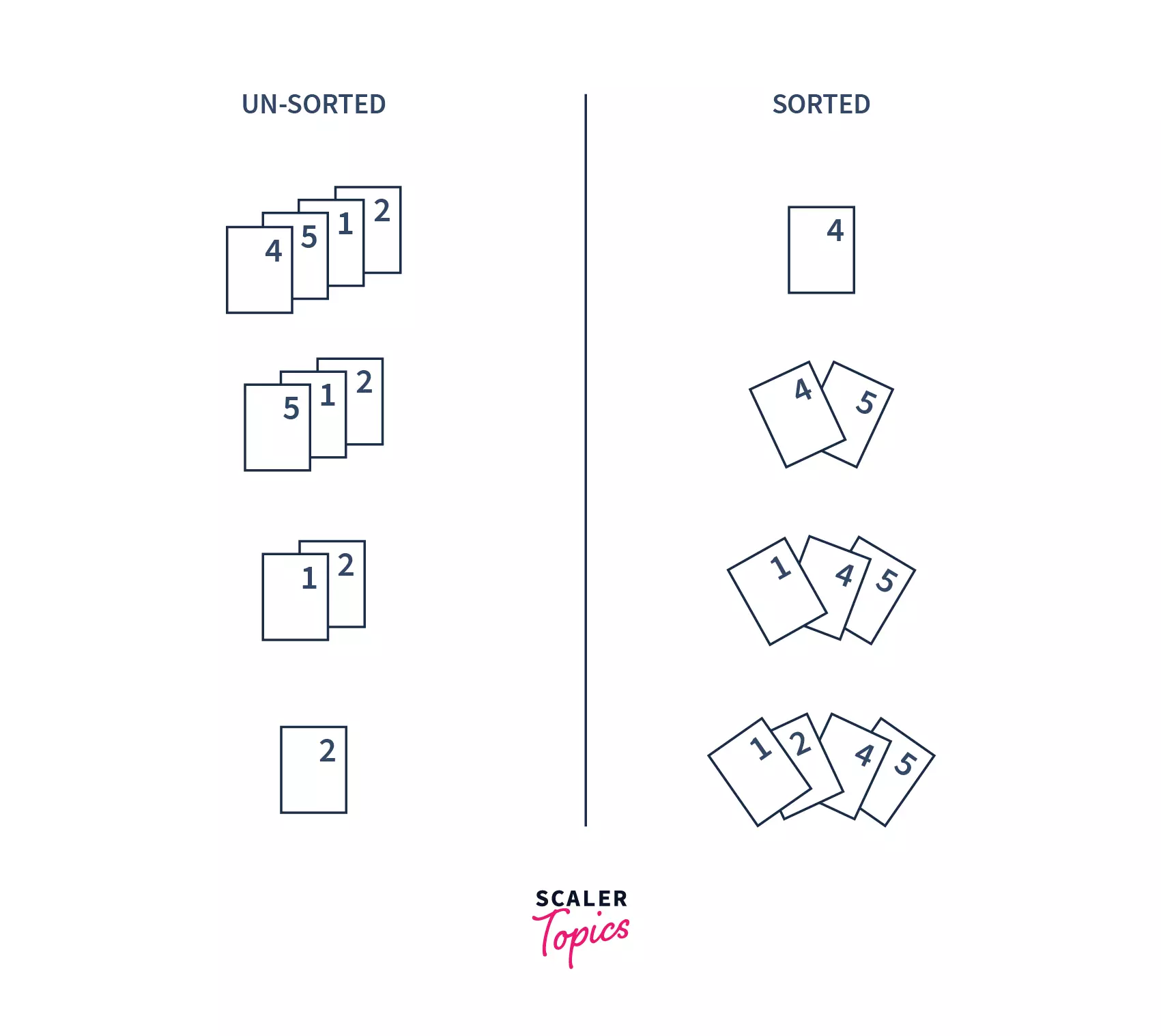
To understand insertion sort, let us first understand one analogy. Insertion sort is performed, just like we sort a deck of cards in any card game.

Suppose, you have a set of cards. Initially, you have one card in your hand. Now, you pick one of the cards and compare it with the one in your hand. If the unsorted card is greater than the card in hand, it is placed on the right otherwise, to the left. In the same way, you will take other unsorted cards and put them in their right place.

• Insertion sort is a sorting algorithm that places an unsorted element at its correct place in each iteration.
• It builds the sorted list one element at a time by comparing each item with the rest of the items of the list and inserting it into its correct position.

Working of insertion sort

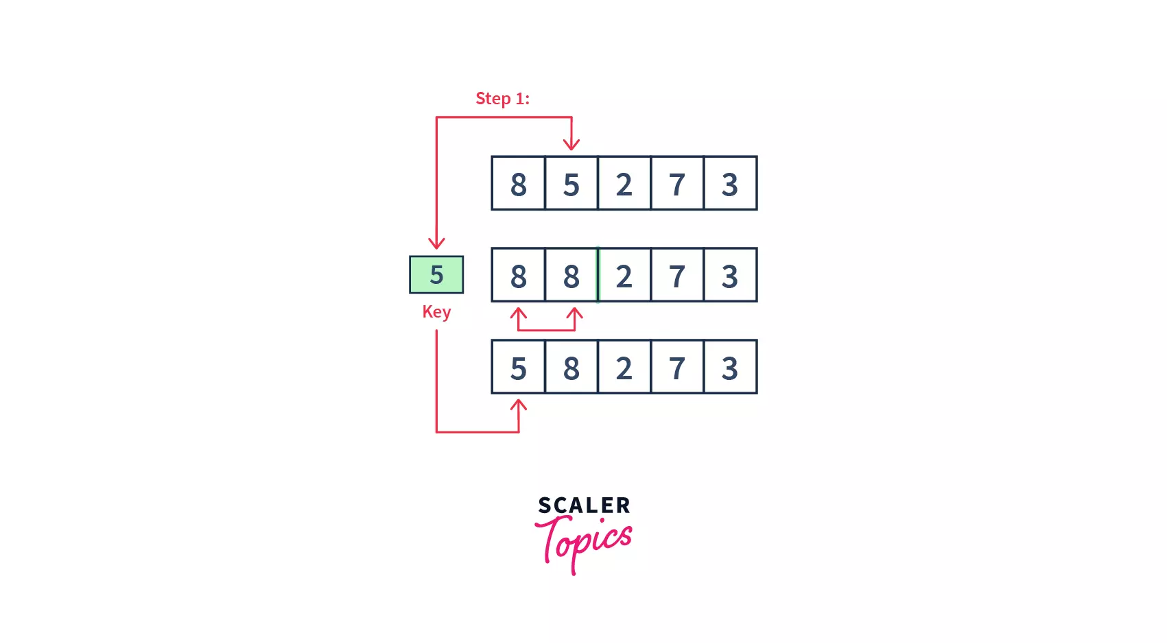
• Firstly, we assume that the first element is sorted, take the second element, and store it in a key variable.

• Then, we are comparing the key with the first element, if the first element is greater than the key, then the key is placed before the first element. Please note that we have 1 comparison and 1 swap in this iteration.

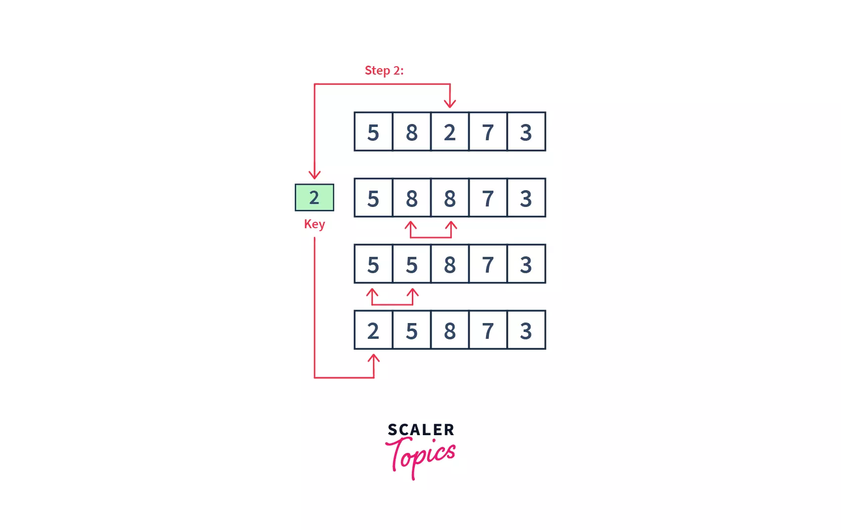
• So, the first two elements are sorted. Similarly, we will perform this step for the third element and compare it with the elements on the left of it. We will keep on moving toward the left, till there is no element smaller than the 3rd element. Then, we will place the third element there(or at the beginning of the array, if it is the smallest element). Please note, in this step, we have 2 comparisons and 2 swaps.

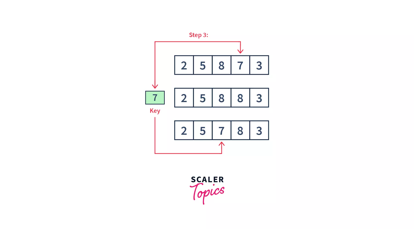
• As we can see, 3 elements of our array are already sorted. Similarly, the 3rd and 4th elements (i.e. 8 and 7) will be compared, and 7 will be sent to its correct position on the left.

• Finally, we have 3 left as our last element. For element 3, 3 comparisons and swaps will be taken to bring it into its correct position.

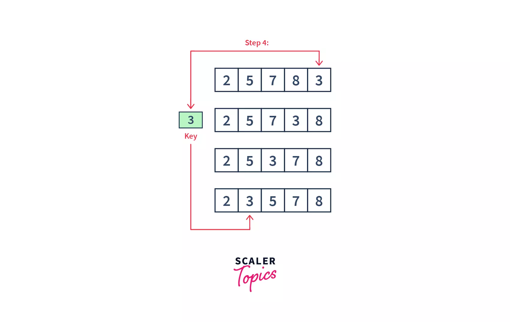
• At the end, all the elements will be sorted in a similar way and the below will be our resultant array. Hence, in 4 passes(iterations), our array got sorted.

Selection Sort

• Selection sort, also known as in-place comparison sort, is a simple sorting algorithm.
• It works on the idea of repeatedly finding the smallest element and placing it at its correct sorted position. It basically selects the smallest element from an unsorted array in each iteration and places that element at the beginning of the unsorted array.
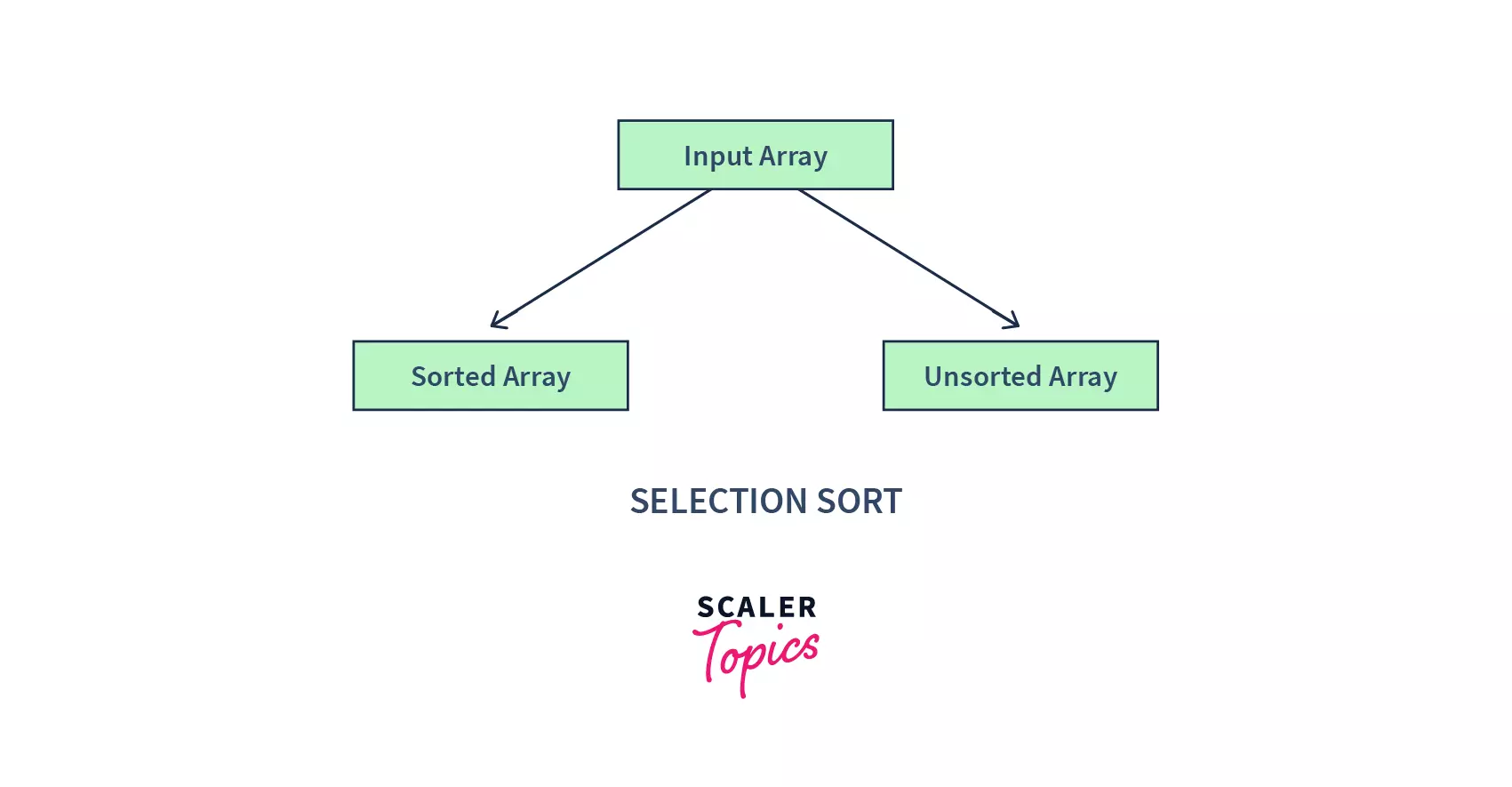
• At any point in time, it maintains two sub-arrays for a given array :
  • Sorted Subarray : The subarray that is already sorted.
  • Unsorted Subarray : The remaining subarray that is unsorted.

With each iteration of the selection sort, we :

• Search for the smallest element in the unsorted sub-array(if we are trying to sort the array in ascending order).
• Place it at the end of the sorted sub-array
• This will continue until we get a completely sorted array, and there is no element left in the unsorted array.

Also, after every iteration, the size of the sorted sub-array increases, and that of the unsorted sub-array decreases.

Working of selection sort :

If we want to sort a list in ascending order, then our algorithm will follow the following steps :

• Initially, our sorted sub-list is totally empty. All the elements are present in the unsorted sub-list. We start with the first element in the array.
• Iterate over the array to search for the smallest element.
• Add this element into the sorted sublist, removing it from the unsorted sublist. We can do that by swapping the smallest element, with the element at whose position we want to store it.
• Repeat the above steps until all the elements from the unsorted sublist are moved to the sorted sublist, and the unsorted subarray becomes empty.

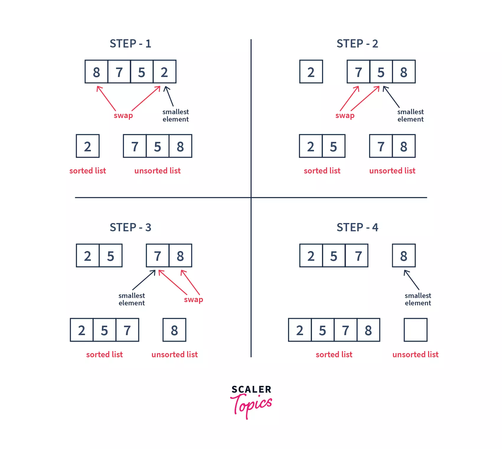
• We had 4 elements in the list, and we got the sorted list in 3 swaps. With this, we may conclude that to sort a list of size n, we need to perform (n – 1) iteration.
• During the first iteration, the smallest element (2 in this case) was selected and added to the sorted sublist. Element 8 swapped its position with 2. Similarly, after each iteration, the smallest among the unsorted elements was placed at its position.
• We can also see that with each iteration, 1 element is stored in its correct position, or getting sorted.

Selection sort pseudocode

Code :

Explanation :

• First, we run a loop through the length of our list.
• Then, we initialize a variable min_index, with the current element's index.
• Our second loop, runs from the next element, which min_index is pointing to, till the end of the list.
• If we find any element, lesser than our current element, we store its position into min_index.
• Then swap values of minimum and current element.
• Continue till all the elements get sorted

Time and space complexity analysis

In selection sort, basically, we have 2 loops. One to iterate over the entire list and another to iterate over the unsorted list. For $n$ elements, the first loop will run $n$ times, and the inner loop runs $n$ times, each time the outer loop runs. Hence, the worst-case time complexity becomes $O(n^2)$

• Worst Case : $O(N^2)$ When we want to sort in ascending order and the array is in descending order then, the worst case occurs. Then, we might need to make $n^2$ comparisons.

• Average Case : $O(N^2)$ When the array is in a jumbled order, then also, roughly we might need around $n^2$ comparisons, so in Big-Oh terms, the complexity becomes $O(N^2)$

• Best Case : $O(N^2)$ When the array is already sorted, then the best case occurs. But we have two loops that will run, irrespective of the value of the elements. So, we will always make $n^2$ comparisons.

• Space complexity : $O(1)$ Space complexity is O(1) because only the temporary variable min_index is used.

Merge Sort

• Merge sort is one of the most efficient sorting algorithms .
• It is based on the `divide and conquers approach, which is a very powerful algorithm.

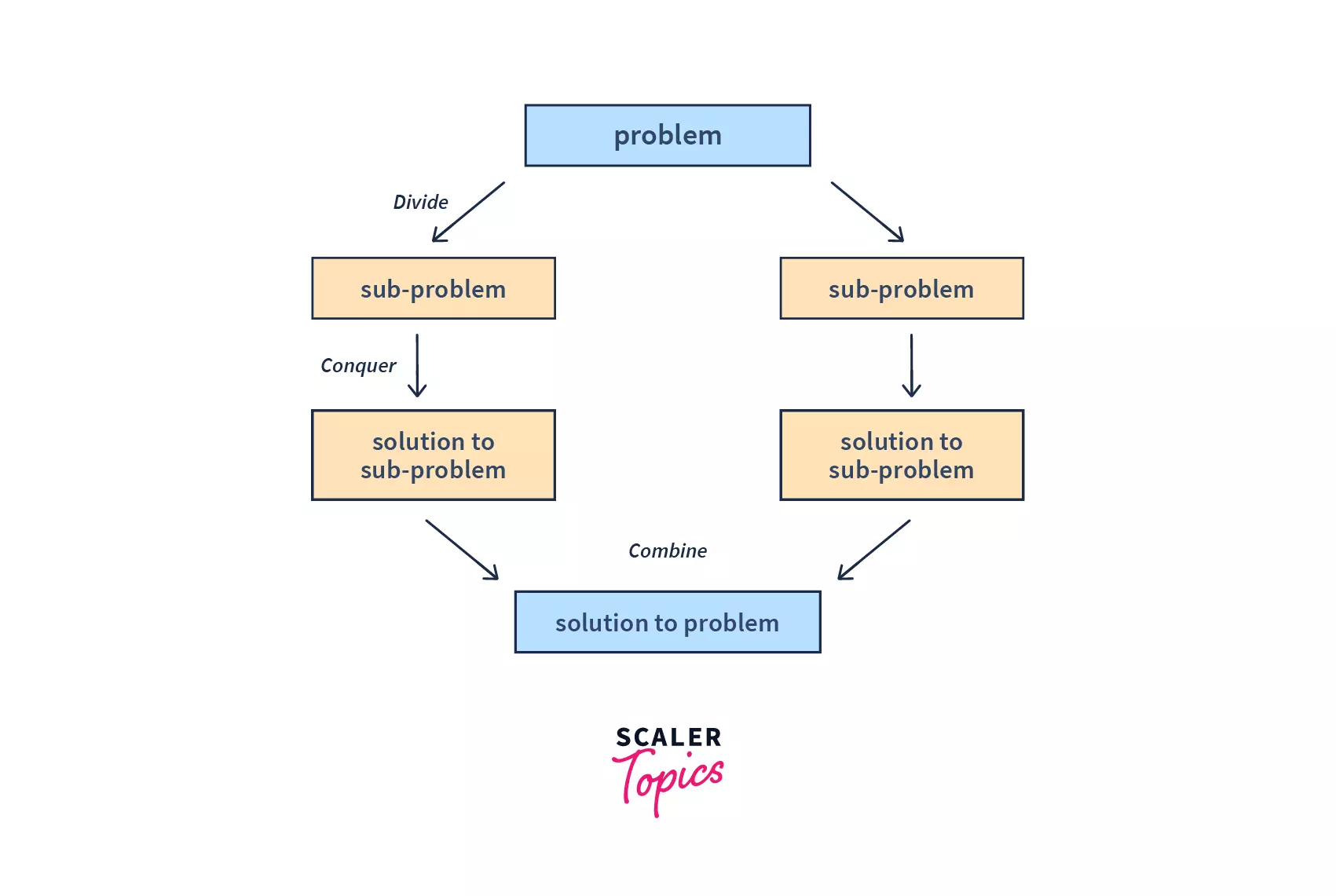
• The divide and conquer algorithm is based on recursion. Recursion breaks down a problem into sub-problems, till a point where the base condition is met or no further sub-problems can be broken into.
• Divide and conquer works in a similar manner:
  • It divides the original array into smaller sub-parts, representing a sub-problem. The sub-problem is similar to the original problem but more simple.
  • Then, it solves those sub-problems recursively.
  • Finally, the solution to those sub-problems are combined to get the result of our original problem

Divide & conquer strategy in merge sort

Suppose, we need to sort an array Arr[]. We can say, that a sub-problem may be considered as sorting a part of the array, starting from any index s(start) and ending at any index e(end). So, we need to sort the array Arr[s...e]. Let us see, how divide and conquer can help us with this problem.

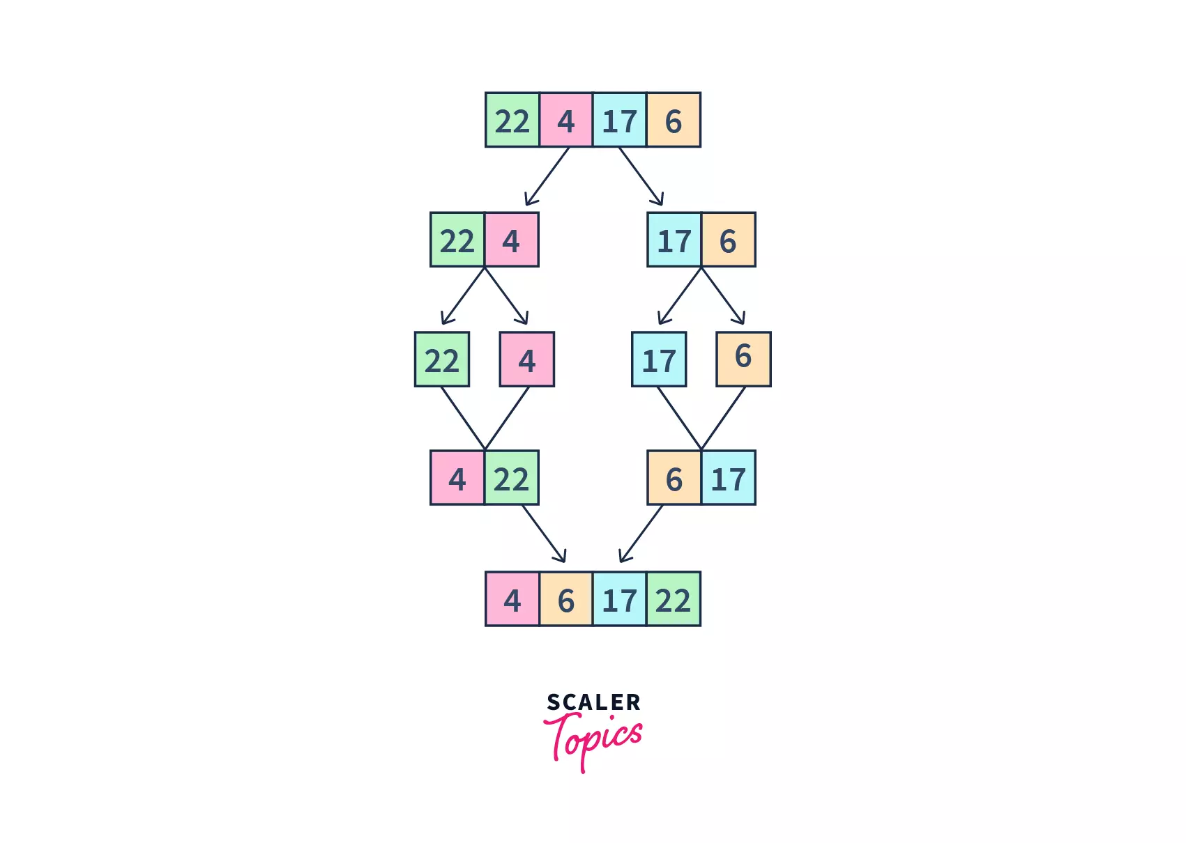
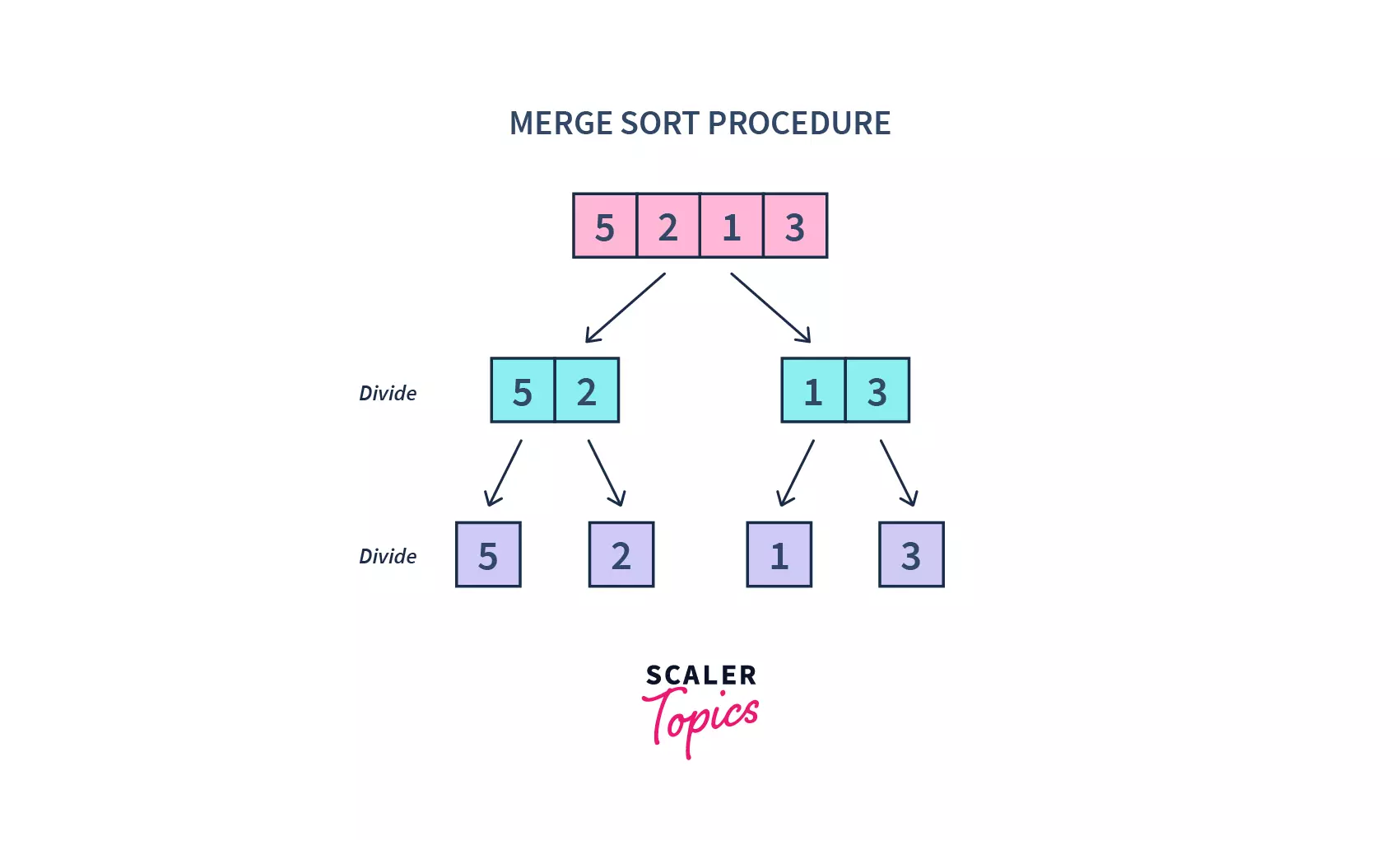
Divide : Suppose m is the mid-point of s and e, then we can split the sub-array Arr[s,e] into two arrays Arr[s,m] and Arr[m+1,e].

Conquer : In the conquer step, we try to sort both the subarrays Arr[s,m] and Arr[m+1,e] and continue this till we have other sub-arrays left. In other words, we do this till we reach the base case. We keep on dividing the sub-arrays and sorting them.

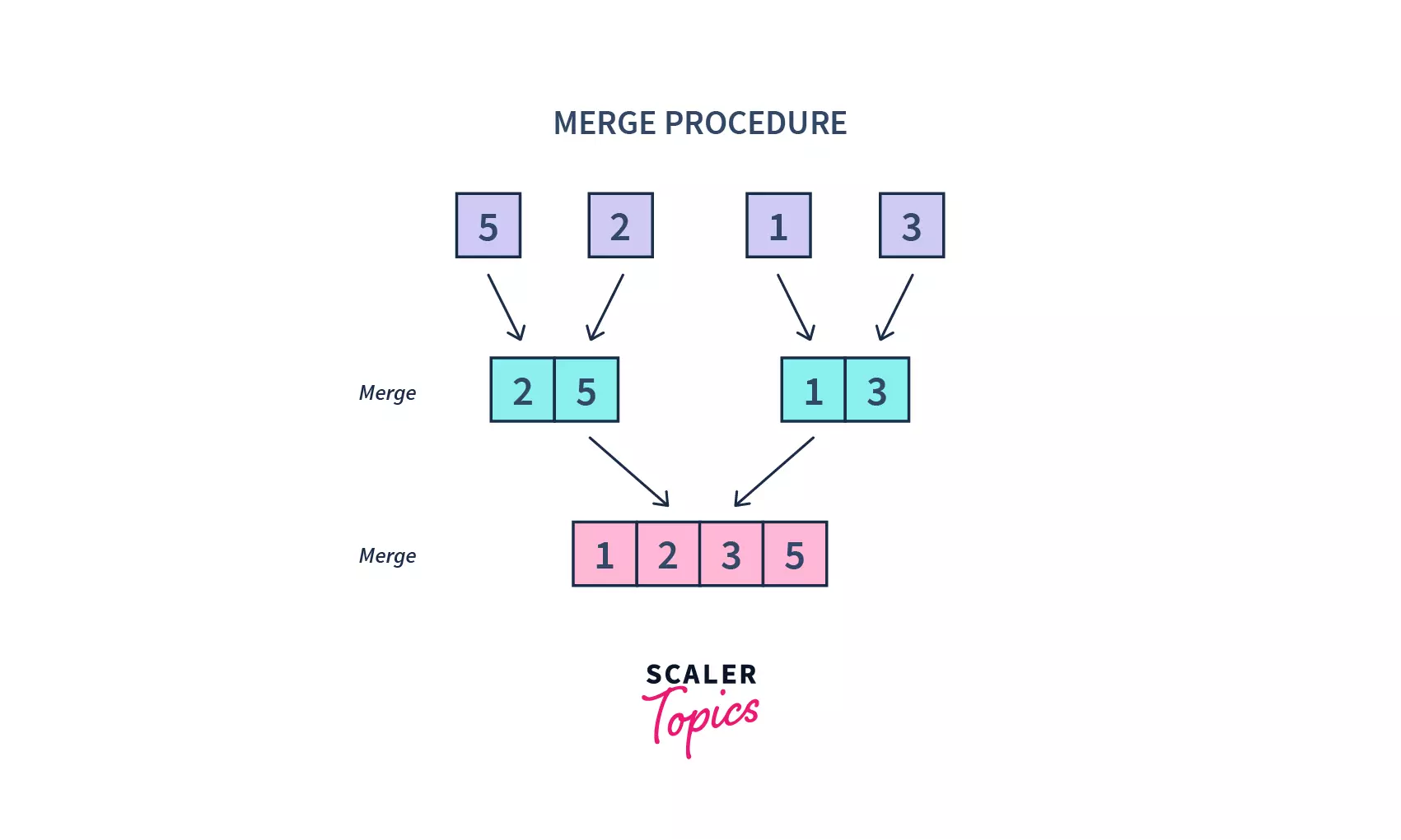
Combine : Once the conquer step has reached the base step and two sorted subarrays Arr[s,m] and Arr[m+1,e] for array Arr[s..e] have been obtained, we combine the results by creating a sorted array Arr[s..e] from two sorted subarrays Arr[s,m] and Arr[m+1,e].

Merge sort algorithm

• We can call the above algorithm with MergeSort(A, 0, length(A)-1).
• We keep a base case, where we check if the start index is larger than the end index, where our recursive calls will terminate.
• We store our mid-value of the index in $m$.
• The MergeSort function divides an array into two halves repeatedly, till we attempt to perform MergeSort on a subarray of size 1, i.e. s == e.

• A merge function is then called on the sorted arrays to combine them into larger arrays until the whole array has been merged. And hence the resultant array is sorted.

Code :

Explanation :

• We divide our array into sub-arrays, find the midpoint and send the sub-arrays to the mergeSort function for further division of the array.
• Once our base case is met, we merge our divided arrays using our merge logic
• In our merge logic, firstly, we compare elements of both the arrays, and whichever is smaller is appended to our array(for ascending order).
• Once it is terminated from the loop, we append the remaining elements from either the left sub-array or right sub-array, to our resultant array.

Time and space complexity analysis

Whenever we divide a number into half in every step, it can be represented using alogarithmic function, which is $log (n)$, and the number of steps can be represented by $log(n+ 1)$(at most). Merge sort always divides the array into two halves and takes linear time to merge them. To merge $n$ elements, $O(n)$ will be required. Hence, the time complexity of Merge Sort is $O(NlogN)$ in all the 3 cases (worst, average and best).

• Worst Case : $O(NlogN)$
• Average Case : $O(NlogN)$
• Best Case : $O(NlogN)$
• Space complexity : $O(N)$ Space complexity is $O(1)$ because only 1 temporary variable min_index is used.
• Stable sort : It is a stable sort, which means the "equal" elements are ordered in the same order in the sorted list.

Quick Sort

• Quicksort, also known as partition-exchange sort, is an in-place sorting algorithm.
• It is a divide-and-conquer algorithm that works on the idea of selecting a pivot element and dividing the array into two subarrays around that pivot.

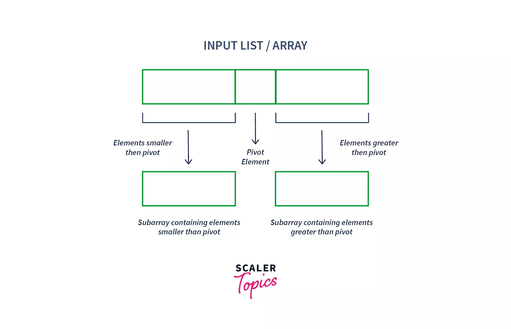
• The array is split into two subarrays. One subarray contains the elements smaller than the pivot element, and another contains the elements greater than it.
• At every iteration, the pivot element is placed at its correct position that it should have in the sorted array.
• This process of selecting the pivot element and dividing the array into subarrays is carried out recursively until all the elements in the array are sorted

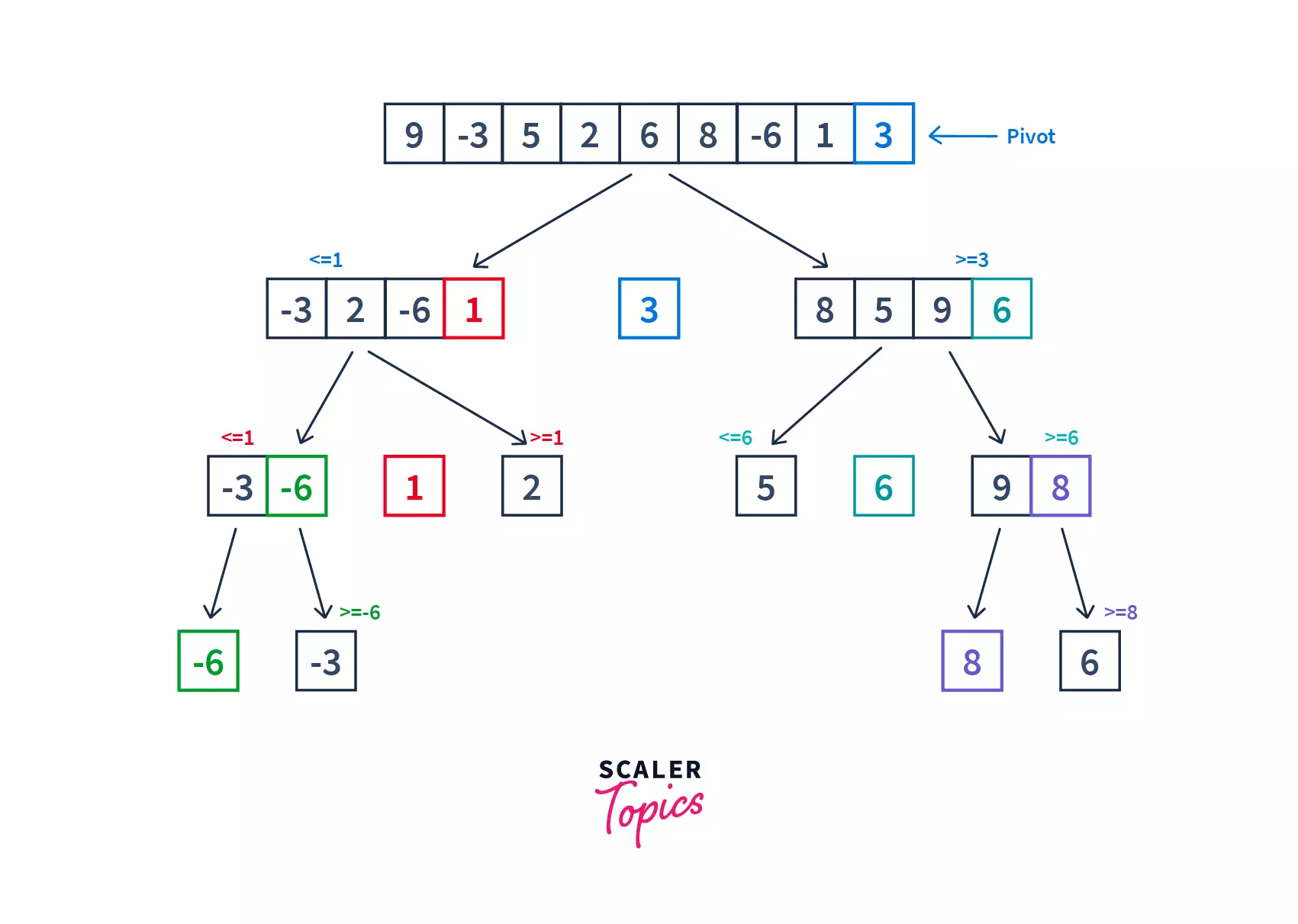
Working of quicksort :

Quick sort first selects a pivot element and partitions the list around the pivot, putting the smaller elements into a low array and all the larger element into a high array. The dividing of the list is known as partitioning the list. Similarly, it keeps on partitioning the lower and the higher array, until each subarray contains a single element. After that, the single element is already sorted and hence combined to form the final array.

Pseudocode for partitioning the array :

Pseudocode for quicksort function :

Time and space complexity analysis

• Worst Case : $O(N^2)$ When the array is sorted, and the pivot always picks the greatest or smallest element, it occurs. Hence, the pivot element lies at an extreme end of the sorted array. One sub-array is always empty and another sub-array contains n - 1 element. So, quicksort is called only on this sub-array.
• Average Case : $O(NlogN)$ When the array is in a jumbled order, then the pivot is near the middle element hence it occurs.
• Best Case : $O(NlogN)$ It occurs when the pivot is almost in the middle of the array, and the partitioning is done in the middle
• Space complexity : $O(1)$ The space complexity is calculated on the basis of space used by the recursion stack. In the worst case, the space complexity of quicksort is $O(n)$ because n recursive calls are made. And, the average space complexity of a quick sort algorithm is $O(logn)$.

Heap Sort

Before learning Heap Sort, let's first understand what is a Heap Data Structure. Heap is a special tree-based data structure. A binary tree is said to follow a heap data structure if

• It is a complete binary tree.
• The parent node of the tree is greater than its left and right child nodes. Then it is a max-heap. On contrary, if the parent node is always smaller than its children, it is a min-heap.

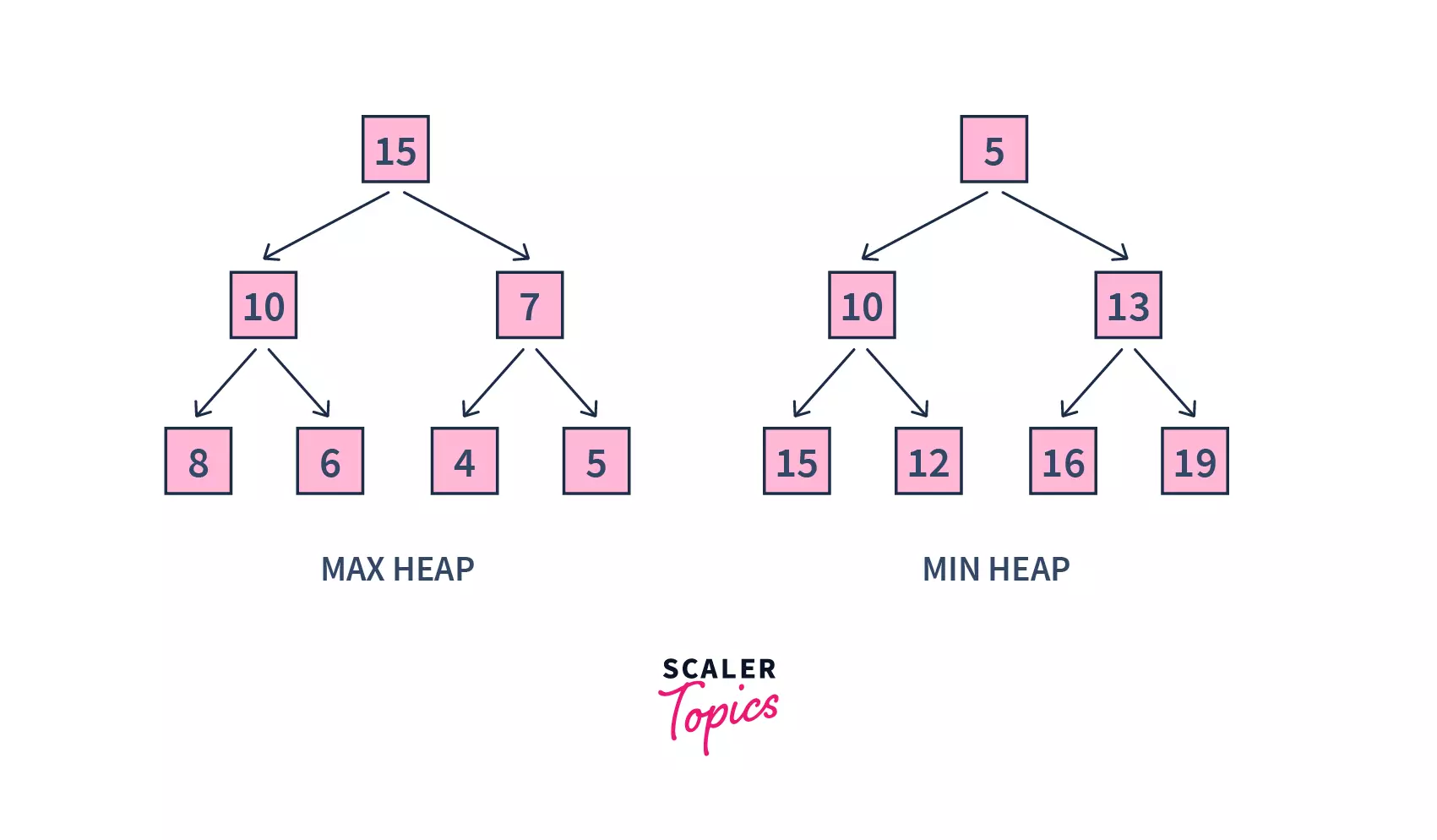
In the above figure, in the case of max-heap, the parent node's value is always greater than the child node's value. Whereas in min-heap, the reverse happens.

Heap sort works by visualizing the elements of the array as this special kind of complete binary tree called a heap.

Relationship between Array Indexes and Tree Elements There is a special relationship between the array indexes and complete binary tree nodes.

• If the index of any element in the array is $i$, the element in the index $2^i +1$ will become the left child and the element in the $2^i+2$ index will become the right child.
• The parent of any element at index $i$ can be given by the lower bound of $(i-1)/2$.

Max-heap : As we discussed above, max-heap is a complete binary tree in which the value in each internal node is greater than or equal to the values in the children of that node.

Working of heapsort

Heap sort follows the below steps to sort an array in ascending order –

• For an array, create a max-heap by visualizing all the elements of the array in a binary tree.
• Heapify is the process of rearranging the elements to form a tree that maintains the properties of a heap. Heapify the binary tree using the elements in the unsorted region of the array.
• Here, we have to build a max-heap since we want to sort the array in ascending order. Heapifying helps us in maintaining the property that every node should have greater value than its children nodes.
• Once the heap is formed, delete the root element from the heap, and add this element to the sorted region of the array. Here, since we are removing the root element from a max-heap, we will obtain the largest element from the unsorted region each time an element is removed
• Repeat steps 2 & 3 until all the elements from the unsorted region are added to the sorted region.

Heapify Algorithm :

Algorithm for Heap Sort :

Time and space complexity analysis

The height of a complete binary tree containing n elements is $log(n)$. In the worst case, we may need to move an element from the root to the leaf node with around $log(n)$ comparisons and swaps. During build_max_heap, we do that for $n/2$ elements so the worst-case complexity of the build_heap step is $nlog(n)$. While sorting, we exchange the root element with the last element and heapify the root element taking $log (n)$ worst time, because we may have to bring the element from the root to the leaf. Since we repeat this $n$ times, the heap_sort step is also $nlog (n)$.

• Worst Case : $O(NlogN)$
• Average Case : $O(NlogN)$
• Best Case : $O(NlogN)$
• Space complexity : $O(1)$

Radix Sort

Let us first take an example to understand radix sort. Suppose, we have an array of 5 elements. Firstly, we will sort their values based on the value of their unit place. Then, we will sort the value of their tenth place. We will continue to do this till the last significant place of the numbers.

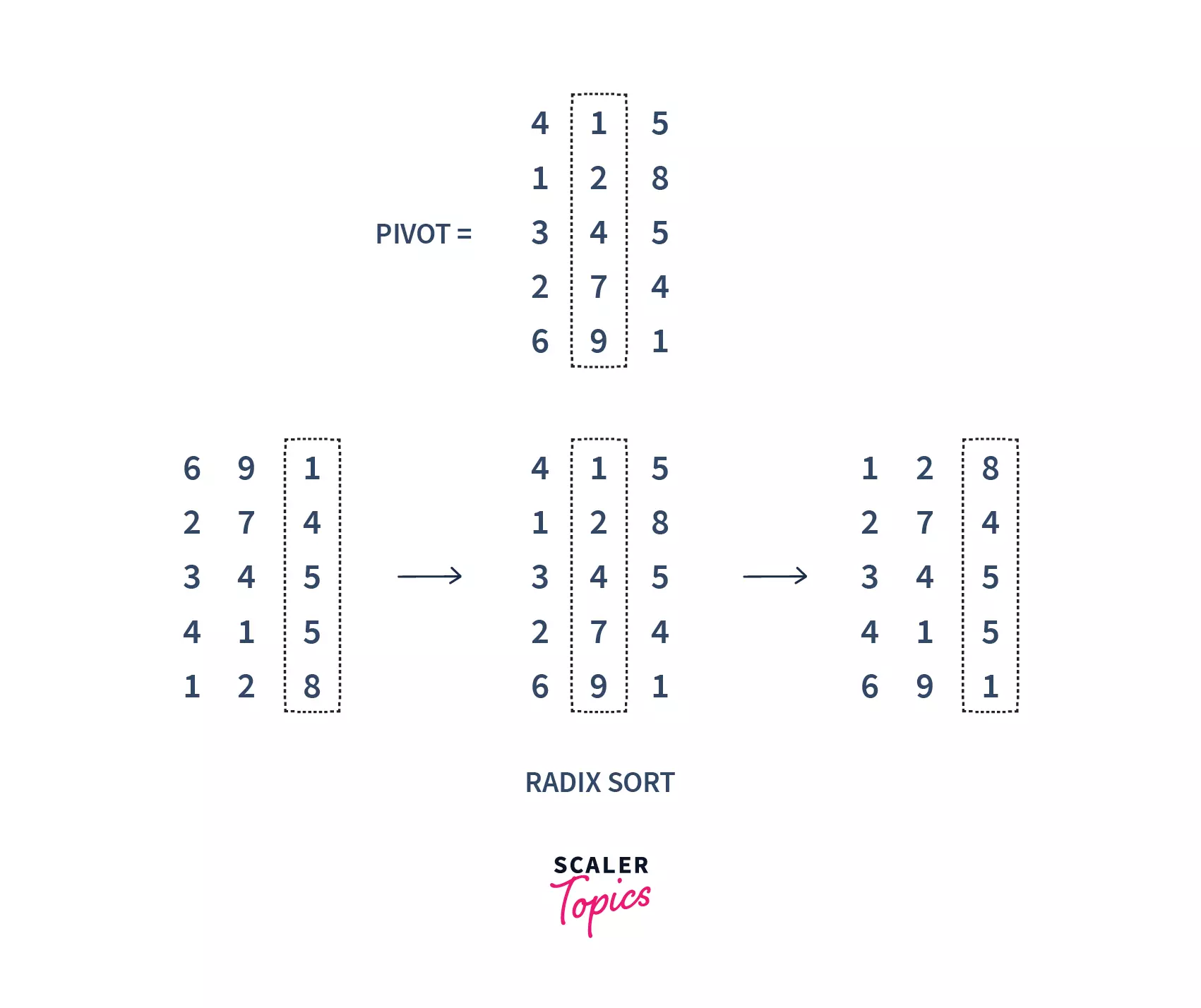
In the above image, we first sort the numbers on the basis of the last digit(unit's place), followed by the digit at 10's place, and so on. Finally, we get our array sorted.

Radix sort algorithm

Explanation : The below given is the general working of the Radix Sort.

• Firstly, we need to get the maximum number of digits of our array. For that, we will find our max element and find the number of digits. For example, in our above array = [112, 126, 335, 445, 457, 841], max num is 841 and the number of digits is 3. So, the loop should go up to hundreds of places (3 times).
• Next, we will visit the significant places one by one. We can sort these digits using any stable sorting technique, for ex. we have used counting sort in our code. And sort the elements based on the unit's place.

• Next, we will sort on the basis of 10's place :

• Next, we will sort on the basis of 100's place :

• Finally, we got our sorted result.

Time and space complexity analysis

Radix Sort takes $O(n+b)$ time where b is the base for representing numbers, for example, for a decimal system, b is 10. However, for the radix sort that uses counting sort as an intermediate stable sort, the time complexity is $O(d(n+k))$.

• Worst Case : $O(n+b)$
• Average Case : $O(n+b)$
• Best Case : $O(n+b)$

The total space used is $number$ $of$ $digits$ $* (n + base)$. If total digit are constant, the space complexity becomes $O(n+base)$. Hence the space complexity of Radix Sort is $O(n+b)$.

• Space complexity : $O(n+b)$

Bucket Sort

• Bucket sort is a sorting technique that uses the Scatter-Gather-Approach to sort the array.
• It works by dividing the unsorted array of elements into several groups called buckets.
• The groups(buckets) are then sorted by using any sorting algorithm. Or, we can apply the bucket algorithm to sort them.
• Finally, the sorted buckets are combined to form a final sorted array.

Working of bucket sort:

Let us understand the general working of bucket sort :

• Consider this is our array

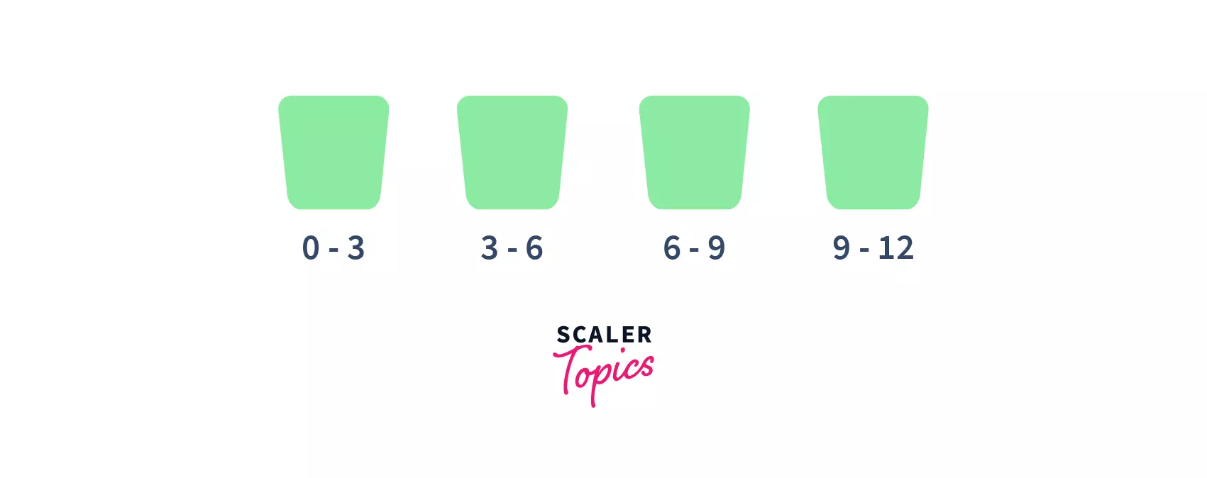
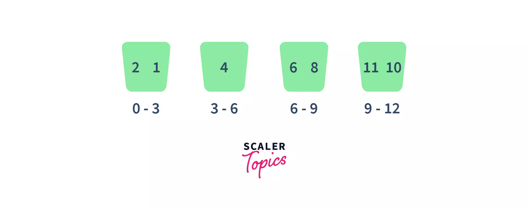
• First, partition the given range of numbers into a fixed number of buckets. For example, here we have partitioned into 4 buckets of the given ranges each.

• After that, put every element into its appropriate bucket, in such a way that each element lies within the given range.

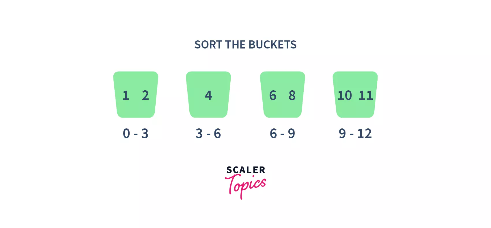
• Then sort each of the buckets by applying any suitable sorting algorithm.

• Finally, combine all the sorted buckets.

Code :

Time and space complexity analysis

The time complexity of Bucket Sort highly depends upon the size of the bucket list and also the range over which the elements in the array/list have been distributed. Because, if the elements in the array don't have much mathematical difference between them, then most of the elements might get placed into the same bucket, increasing the complexity. For $k$ buckets and $n$ elements, the overall time complexity of bucket sort is $O(n+b)$.

• Worst Case : $O(n^2)$ This will happen when all of the elements will be stored inside the same bucket. Hence sorting them, using a normal algorithm, such as bubble sort, may take $O(n^2)$ time.
• Average Case : $O(n+b)$ The average case occurs when the elements are distributed randomly in the list, considering there are n elements spread across b buckets.
• Best Case : $O(n+b)$ It occurs when the number of elements spread across each bucket is the same, considering there are $n$ elements spread across $b$ buckets.
• Space complexity : $O(n+b)$ The space complexity for Bucket sort is $O(n + b)$, where $n$ is the number of elements and $b$ is the number of buckets.