Gradient Descent in Machine Learning: Intuition, Math & Code
Most explanations of gradient descent pick a lane. The intuition-only pages give you a nice mountain metaphor and send you off with no idea how to actually implement anything. The math-heavy pages throw a wall of partial derivatives at you and assume you'll figure out why any of it matters. Neither approach really works if you're trying to get this to click before an interview, or before your next model just refuses to train properly.
This piece does all three layers with one running example: fitting a straight line to five data points. Same numbers, all the way from the plain-English version through to working NumPy code. If a number shows up in a table below, it was actually computed, not estimated.
What Is Gradient Descent in Machine Learning?
Gradient descent is an iterative optimization algorithm that minimizes a loss function by repeatedly moving a model's parameters in the direction that reduces error the fastest. That's the whole idea. Everything else in this article is detail on top of that one sentence.
It's not one specific technique buried inside machine learning, it's closer to the engine room. Linear regression uses it. Every neural network you've heard of uses some flavour of it. Whenever people say a model "learned" something, what actually happened underneath is gradient descent nudging numbers in a slightly better direction, over and over, until the errors got small enough to stop caring about.
Build an AI-First Career, Master the Complete Skillset
Choose from our industry-leading programs designed for career success
Modern Software and AI Engineering Program
Master full-stack development with AI integration


 +1000 more
Modern Data Science and ML with specialisation in AI
Advanced data science techniques with AI specialization
+1000 moreAdvanced AIML with Specialisation in Agentic AI
Deep dive into AIML with focus on Agentic systems
+1000 moreDevOps, Cloud & AI Platform Engineering
Build and manage AI-powered cloud infrastructure
+1000 moreAI Engineering Advanced Certification by IIT-Roorkee
Premier AI engineering certification from IIT-Roorkee

AI Forward Deployed Engineer Program
Full-stack engineering, production AI and client-facing consulting
+1000 moreStop learning AI in fragments—master a structured AI Engineering Course with hands-on GenAI systems with IIT Roorkee CEC Certification
:::


AI Engineering Course Advanced Certification by IIT-Roorkee CEC
A hands on AI engineering program covering Machine Learning, Generative AI, and LLMs - designed for working professionals & delivered by IIT Roorkee in collaboration with Scaler.
Enrol Now
The Intuition: Descending a Mountain in Fog
Picture standing on a mountain at night with zero visibility. You want to get to the lowest point in the valley, but you can't see more than your own feet.
• You feel which way the ground slopes under you
• You take a step in the downhill direction
• You repeat, checking the slope again each time, until the ground feels flat
That's genuinely most of gradient descent. No calculus needed to get the idea, just the willingness to keep checking your footing and moving accordingly. Here's how that maps onto the actual algorithm:
| On the mountain | In gradient descent | What it means |
|---|---|---|
| Your altitude | The loss, J(theta) | How wrong the model currently is |
| Your position | The parameters, theta (w, b) | The current guess for the model's weights |
| The slope under your feet | The gradient | Which direction makes things worse fastest, you step the opposite way |
| Your stride length | The learning rate, eta | How far you move on each step |
| Reaching the valley floor | Convergence | Loss stops meaningfully decreasing |
One thing the metaphor undersells: in real ML problems you're not walking down a mountain in two dimensions, you're doing it in however many dimensions your model has parameters. A small neural network might have thousands. GPT-scale models have billions. The fog metaphor still holds, it's just fog in a space nobody can actually picture, which is a fun thing to sit with for a second.
Stop learning AI in fragments—master a structured AI Engineering Course with hands-on GenAI systems with IIT Roorkee CEC Certification
:::
AI Engineering Course Advanced Certification by IIT-Roorkee CEC
A hands on AI engineering program covering Machine Learning, Generative AI, and LLMs - designed for working professionals & delivered by IIT Roorkee in collaboration with Scaler.
Enrol NowThe Role of the Cost Function
Before you can walk downhill, you need to know what "downhill" even means, and that's the job of the cost function (also called the loss function). It's a single number that says how wrong the model currently is. Lower is better. Gradient descent's entire job is pushing that number down.
For the line-fitting example running through this piece, that function is mean squared error:
J(w, b) = (1/n) * sum((w*x_i + b - y_i)^2)
A quick word on why it needs to be differentiable: gradient descent works by computing slopes, and you can't take the slope of a function that has hard corners or discontinuities everywhere. MSE is smooth and bowl-shaped for linear regression, which is exactly what makes this whole approach work cleanly here.
The Math: The Gradient Descent Formula Explained
Here's the update rule, in full:
theta_new = theta_old - eta * grad(J(theta))
Reading it left to right, in plain words:
• theta is whatever parameter you're updating (w or b in our example)
• eta (the learning rate) controls how big a step you take
• grad(J(theta)) is the gradient, the direction of steepest increase in loss
• Subtracting it moves you in the opposite direction, downhill, toward lower loss
For our MSE cost function, the partial derivatives with respect to w and b work out to:
dJ/dw = (2/n) * sum((w*x_i + b - y_i) * x_i) dJ/db = (2/n) * sum(w*x_i + b - y_i)
If deriving those from first principles feels shaky, that's just a calculus gap, not an ML gap, and it's worth closing separately. Scaler's free Maths for Machine Learning course covers exactly this kind of derivative work if you want the refresher before going further.
How Scaler Transformed Careers in Different Fields
Scaler learners achieved 2.5x salary growth with average post-Scaler CTC reaching ₹23L.
 Google
 Amazon
 Microsoft
 Flipkart
 Adobe1200+ more
Gradient Descent Step by Step: A Worked Example
Here's the running example: fitting y = wx + b to five points.
• Data: (1, 2.9), (2, 5.2), (3, 6.8), (4, 9.3), (5, 10.9)
• Starting point: w = 0, b = 0 (about as wrong a guess as you can make)
• Learning rate: eta = 0.01
Three iterations, by hand, all numbers to four decimal places:
| Iteration | w, b (start) | Loss (MSE) | Gradients (dw, db) | w, b (updated) |
|---|---|---|---|---|
| 1 | 0.0000, 0.0000 | 57.3980 | -50.1600, -14.0400 | 0.5016, 0.1404 |
| 2 | 0.5016, 0.1404 | 33.4764 | -38.2824, -10.7496 | 0.8844, 0.2479 |
| 3 | 0.8844, 0.2479 | 19.5360 | -29.2153, -8.2377 | 1.1766, 0.3303 |
Loss falls from 57.3980 to 19.5360 in three steps. It doesn't reach zero, and it shouldn't yet, this is three iterations out of what ends up being hundreds before it settles. Run the same setup for 1,000 epochs and w and b converge to roughly 2.0138 and 0.9764, which lines up almost exactly with the closed-form least-squares solution (w = 2.0100, b = 0.9900) you'd get by solving the linear regression problem directly. Gradient descent isn't cheating its way to an answer, it's crawling toward the same one algebra would give you, just without needing to invert a matrix.
Learning Rate: The Most Important Hyperparameter
Get the learning rate wrong and nothing else in this article matters.
• Too small: training crawls. Technically correct, practically useless if it takes 200,000 epochs to get anywhere.
• Too large: each step overshoots the minimum, loss starts bouncing around, and it can genuinely diverge (loss going up instead of down, which is a special kind of frustrating to debug at 1am).
• Just right: steady, smooth decrease, converges in a reasonable number of steps.
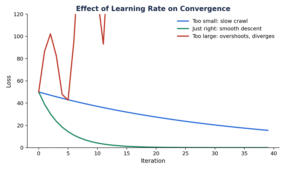
In practice almost nobody picks one fixed learning rate and walks away. Learning rate schedules (decaying the rate as training progresses) and adaptive methods are both common enough that "just tune eta once" is more of a teaching simplification than something you'd actually do on a real project.
Types of Gradient Descent
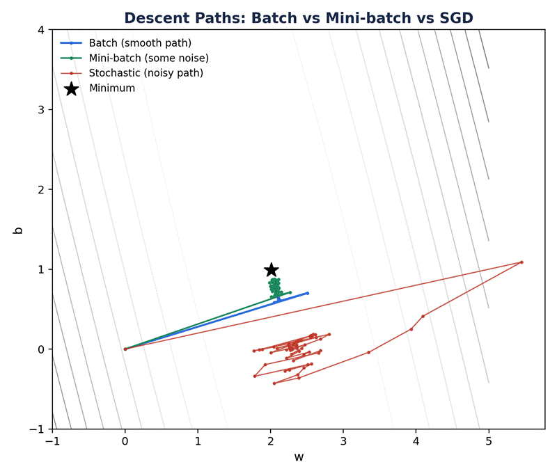
Three variants, and they mostly differ on one question: how much data do you look at before taking a single step?
| Type | Update frequency | Memory use | Convergence path | When to use |
|---|---|---|---|---|
| Batch | Once per full pass over the dataset | High, needs the whole dataset in memory | Smooth, stable, slow | Small datasets that fit comfortably in memory |
| Stochastic (SGD) | Once per single sample | Very low | Noisy, jittery, but fast and can escape shallow local minima | Huge datasets, online learning |
| Mini-batch | Once per small batch (32 to 256 samples, typically) | Moderate | Some noise, mostly stable, GPU-friendly | Basically everything in deep learning today |
Worth saying plainly since a lot of pages dance around it: mini-batch is what deep learning actually runs on. Not batch, not pure SGD. Mini-batch gets you a reasonable amount of the stability batch gives you, most of the speed SGD gives you, and it happens to map extremely well onto how GPUs like to chew through data in parallel chunks.
Turn Learning into Career Growth
Challenges: Local Minima, Saddle Points, and Plateaus
Vanilla gradient descent can get stuck, and not always for the reason people assume.
• Local minima: a dip that looks like the bottom but isn't the actual lowest point anywhere on the surface.
• Saddle points: flat in some directions, sloped in others, so the gradient shrinks toward zero even though you haven't actually found a minimum.
• Plateaus: stretches where the loss surface is nearly flat everywhere, so progress just crawls.
Here's the part that surprises people: in high-dimensional loss surfaces (which is most real neural networks), saddle points vastly outnumber true local minima. Dauphin et al. (2014) made this case directly, and it's part of why modern optimizers spend more design effort escaping saddle points than avoiding local minima, the local-minima problem was never really the main villain in high dimensions. The Deep Learning Book's optimization chapter is the standard reference if you want the fuller mathematical treatment here.
Beyond Vanilla: Momentum, RMSProp, and Adam
Momentum adds a bit of memory to the process, imagine a ball rolling downhill that keeps some of its previous velocity instead of stopping and recalculating direction from scratch at every single step. It smooths out the noisy parts of the path and helps push through small bumps and shallow local dips. Our momentum-based gradient descent page goes deeper into the mechanics if this is the variant you need for a project.
RMSProp and Adam take a different angle: adaptive learning rates, where each parameter effectively gets its own step size based on how its gradients have behaved recently. Adam (Kingma & Ba, 2014) in particular has become close to a default choice in a huge share of modern training setups, combining momentum with per-parameter adaptive rates. It's not always the objectively optimal choice for every problem, but "just use Adam" is a genuinely reasonable starting point rather than a cop-out.
Our optimizers in deep learning page covers the full lineup in more depth than fits here. If you want to actually train models with these instead of just reading about them, Scaler's free Deep Learning course is built around exactly that kind of hands-on practice.
Gradient Descent in Python (From Scratch)
Here's the running example automated, no libraries beyond NumPy:
import numpy as np
x = np.array([1, 2, 3, 4, 5], dtype=float)
y = np.array([2.9, 5.2, 6.8, 9.3, 10.9], dtype=float)
n = len(x)
w, b = 0.0, 0.0
eta = 0.01
epochs = 1000
for epoch in range(1, epochs + 1):
pred = w * x + b
error = pred - y
loss = np.mean(error ** 2)
dw \= (2 / n) \* np.sum(error \* x)
db \= (2 / n) \* np.sum(error)

w \-= eta \* dw
b \-= eta \* db

if epoch % 200 \== 0:
 	print(f'Epoch {epoch}: loss={loss:.4f}, w={w:.4f}, b={b:.4f}')
print(f'Final: w={w:.4f}, b={b:.4f}')
Running that prints roughly this (actual output, not made up for the article):
Epoch 200: loss=0.0451, w=2.0666, b=0.7856
Epoch 400: loss=0.0394, w=2.0388, b=0.8862
Epoch 600: loss=0.0379, w=2.0246, b=0.9373
Epoch 800: loss=0.0375, w=2.0174, b=0.9632
Epoch 1000: loss=0.0374, w=2.0138, b=0.9764
Final: w=2.0138, b=0.9764
That's the entire algorithm in about twenty lines. Everything sklearn's LinearRegression or PyTorch's optimizer objects do is a more general, more optimized version of this exact loop, with a lot more error handling and vectorization tucked away where you don't have to look at it.
Gradient Descent vs Backpropagation
This mix-up comes up constantly, understandably, since the two terms show up together so often they start to blur.
• Backpropagation computes the gradients, it's the process of working out, layer by layer, how much each weight in a neural network contributed to the final error.
• Gradient descent uses those gradients, it's the update rule that actually moves the weights once backprop has handed over the direction to move in.
One computes the "which way is downhill," the other does the "take a step." You genuinely can't have one without the other in a neural network, they're two different stages of the same training loop, not competing techniques. If backpropagation itself still feels fuzzy, our dedicated backpropagation guide is the natural next read, it's built to connect directly back into everything covered here.
Ready to train models end to end? Explore Scaler's AI & ML Program for the structured path from these fundamentals through to production-grade model training.
FAQs
What is gradient descent in simple words? An algorithm that improves a model by repeatedly nudging its parameters in the direction that reduces error the fastest, like walking downhill by always stepping toward the steepest descent.
What are the three types of gradient descent? Batch (entire dataset per update), stochastic (one sample per update), and mini-batch (small batches, the practical default in deep learning).
What is the learning rate in gradient descent? The step size of each update. Too small makes training slow, too large makes the loss oscillate or diverge.
Is gradient descent the same as backpropagation? No. Backpropagation computes the gradients in a neural network, gradient descent uses those gradients to actually update the weights.
Why does gradient descent get stuck? Local minima, saddle points, and flat plateaus can all stall progress. Momentum-based and adaptive optimizers like Adam are largely designed to push through exactly these situations.
Does linear regression use gradient descent? It can. For large datasets, gradient descent is generally preferred over the closed-form normal equation, and it's also the standard way the concept gets taught, since it generalizes to models where a closed form doesn't exist at all.